3. Robust Systems Lab May 28, 2026 11 min

3.8 How to Make Indicators More Stationary

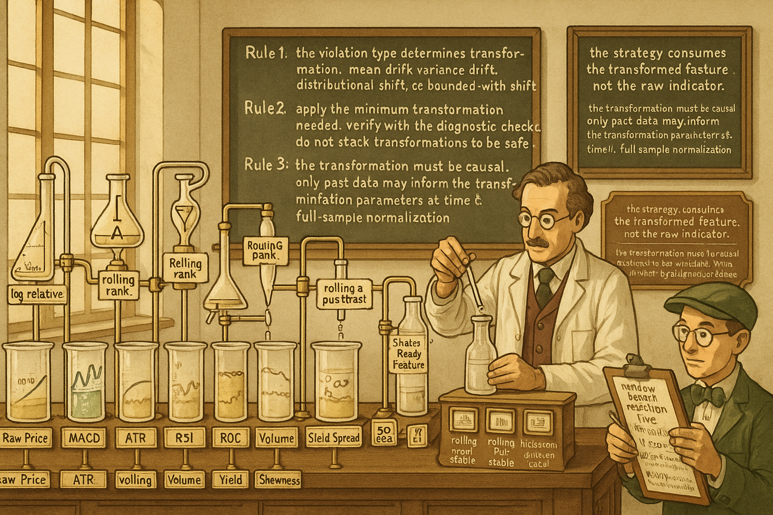
Raw indicators have non-stationary distributions that break threshold rules across decades. Match the violation to the transformation. Eight classes, eight recipes. Verify causally. Do not stack.

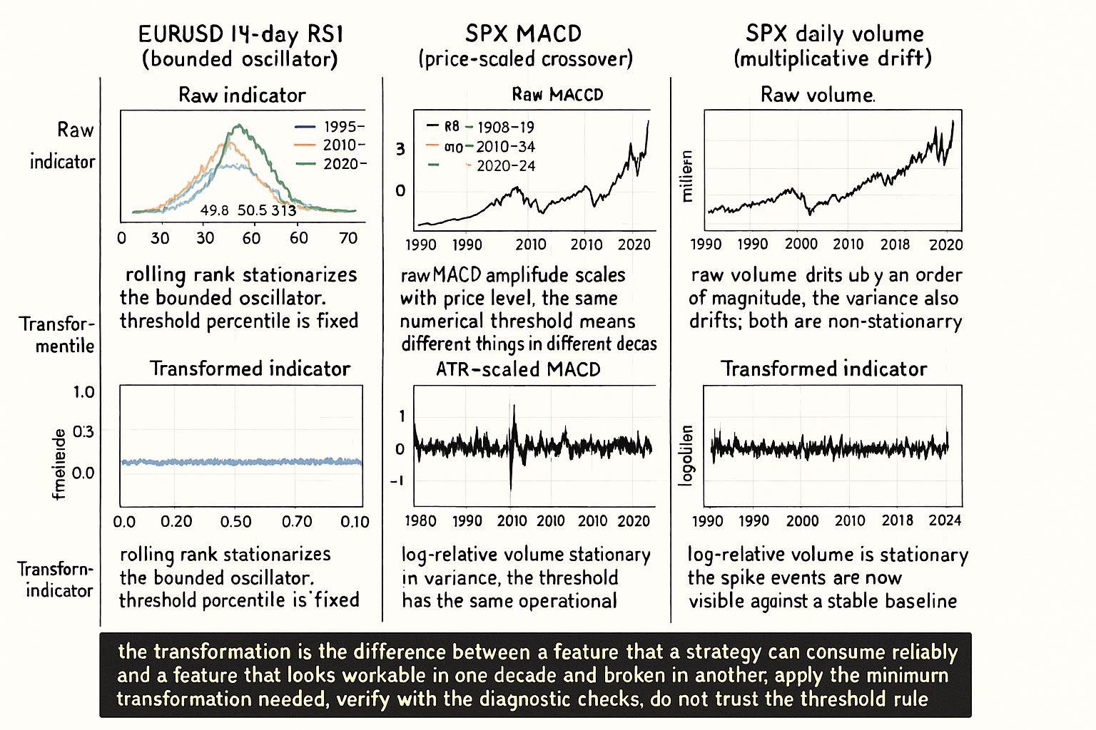
Take the standard 14-period RSI on EURUSD daily across 1995 to 2024. The unconditional histogram of the indicator looks reasonable: a roughly symmetric distribution centered near 50, with most mass between 30 and 70 and tails reaching toward 20 and 80. Slice the same indicator into 5-year windows and the unconditional appearance breaks down. The 1995 to 1999 RSI distribution has median 49.8 and 90th percentile 73. The 2010 to 2014 distribution has median 50.3 and 90th percentile 76. The 2020 to 2024 distribution has median 51.9 and 90th percentile 71. The shifts are small but operationally lethal: a threshold rule "go long when RSI < 30" fires at the 12th percentile of the 1995 to 1999 distribution, the 9th percentile of 2010 to 2014, and the 14th percentile of 2020 to 2024. The same rule selects different fractions of trading days across windows, with different post-trigger return distributions, and the strategy backtest mixes those windows into a single composite estimate that is correct for none of them.

The diagnosis is non-stationarity in the indicator distribution. The fix is to transform the raw indicator into a more stationary form before any threshold rule consumes it. The article "Stationarity: The Word Every Trader Ignores Until It Kills the Strategy" gave five tools at high level. This article gives the practical recipes by indicator class: which transformation matches which indicator, why, and what diagnostic confirms the transformation worked. The next article in the publication ("When Forcing Stationarity Destroys Information") covers the counter-case where over-aggressive transformation destroys the very signal the strategy was supposed to consume.

The transformation pipeline

A four-step workflow that applies to any raw indicator.

Step 1: diagnose the non-stationarity. Plot the indicator's rolling 252-day mean and rolling 252-day standard deviation across the full sample. Plot the indicator's distribution histograms for non-overlapping 4 to 5 year windows. Apply Kolmogorov-Smirnov or Anderson-Darling on consecutive windows. The article "Why OOS Failure Is Often a Stationarity Failure" framed the regime-overlap test machinery; the same machinery applies here at the feature level.

Step 2: identify the violation type. The diagnosis produces one of four patterns. Mean drift (rolling mean moves persistently). Variance drift (rolling std varies by more than 50% across windows). Distributional shape change (the histogram shape changes even if mean and variance are stable). Bounded-but-shifting (the indicator is bounded by construction but the within-bounds distribution shifts).

Step 3: apply the matching transformation. The match between violation type and transformation determines the right tool.

Step 4: verify the transformation. Re-run step 1 diagnostics on the transformed feature. The transformed feature should have approximately stable rolling mean, approximately stable rolling std, and approximately stable histogram shape across windows. If it does not, the transformation was the wrong choice or the underlying indicator has multiple non-stationarity modes.

Recipes by indicator class

Eight common indicator classes, with the matching recipe for each.

Class 1: raw price. Indicators that consume raw price (the price itself, simple moving averages, MA crossovers stated in absolute price units) inherit the unbounded non-stationary level. Recipe: convert to log returns or to log-relative measures (log of price divided by the moving average). The transformation produces a feature that is approximately stationary in mean.

$$ \tilde{X}_t = \log\!\left(\frac{P_t}{\text{MA}_t}\right) \quad \text{instead of} \quad X_t = P_t - \text{MA}_t $$

The log-relative form is invariant to the price level and the percent-deviation interpretation is constant across decades. The article "The Case Against Raw Price Indicators" (covered in Pillar 2) framed this point at the indicator-design level.

Class 2: moving-average crossover differences. Indicators like MACD that compute the difference between two MAs are stationary in mean but the variance scales with the price level (a 50-point MACD signal in a 4000-level SPX is the same percent move as a 1-point MACD in a 80-level SPX). Recipe: divide the MACD-style signal by an ATR or rolling std reference.

$$ \tilde{X}_t = \frac{\text{EMA}_{12}(P) - \text{EMA}_{26}(P)}{\text{ATR}_{14}(P)} $$

The ATR-scaled MACD is approximately stationary in variance across regimes. The article "Why ATR Normalization Is More Than a Volatility Trick" covered this technique in detail.

Class 3: range and volatility indicators. ATR, true range, Parkinson estimator. The raw values scale with the price level (a 50-point true range on SPX 4000 is the same as a 0.5-point true range on SPX 40). Recipe: divide by a longer-window reference (multi-year ATR or by the price level itself).

$$ \tilde{\text{ATR}}_t = \frac{\text{ATR}_{14}(t)}{\text{ATR}_{252}(t)} \quad \text{or} \quad \frac{\text{ATR}_{14}(t)}{P_t} $$

The first form (short ATR / long ATR) is the relative-vol form and is stationary in level by construction (the ratio is dimensionless and its long-run mean is approximately 1.0). The second form (ATR / price) is the percent-vol form and is stationary on multi-decade windows.

Class 4: bounded oscillators. RSI, Stochastics, Williams %R. The raw indicator is bounded but the within-bounds distribution shifts (the example at the top of this article). Recipe: rolling rank or rolling z-score within a moderate window.

$$ \text{rank}_W(X_t) = \frac{\#\{X_{t-i} : i \in [0, W-1], X_{t-i} \le X_t\}}{W} $$

The rolling rank maps the indicator to [0, 1] uniformly within the rolling window. The transformed feature is uniform on its rolling distribution by construction, which makes threshold rules invariant to the within-window distribution shape. The article "Why Indicator Histograms Matter" framed this for the design phase.

Class 5: unbounded momentum / ROC indicators. ROC, MOM, signed cumulative returns over a window. The raw indicator is unbounded and its variance scales with the price-return distribution which is itself non-stationary. Recipe: scale by a forecast or rolling estimate of the return std.

$$ \tilde{X}_t = \frac{\text{ROC}_{20}(P_t)}{\hat{\sigma}_{\text{return}, 20}(t)} $$

The result is a vol-normalized momentum feature whose distribution has approximately stable variance across regimes. The point is that a 5% return in a 8%-vol regime is a different signal than a 5% return in a 18%-vol regime; vol-normalization makes the two comparable.

Class 6: volume indicators. Raw volume is non-stationary in mean (it grows with the long-run growth of trading activity), in variance (volume is heteroskedastic), and often has unit-root properties. Recipe: log-transform first, then subtract a rolling mean.

$$ \tilde{V}_t = \log(V_t + 1) - \overline{\log(V)}_{252} $$

The log handles the multiplicative growth and the heteroskedasticity. The rolling-mean subtraction handles the slow drift in baseline activity. The +1 in the log is a numerical safeguard for zero-volume bars.

Class 7: spread and rate indicators. Yield-curve slopes, credit spreads, FX-cross spreads. The raw indicator is approximately stationary in some regimes and has slow drift in others. Recipe: differencing for the persistent component and rolling z-scoring for the regime-conditional level.

$$ \tilde{X}_t = \Delta X_t \quad \text{(if drift is the issue)} \quad \text{or} \quad z_t = \frac{X_t - \hat{\mu}_t}{\hat{\sigma}_t} \quad \text{(if regime level is the issue)} $$

The choice depends on the diagnostic. If the indicator has a unit root (KPSS rejects, ADF fails to reject), use differencing. If the indicator has slow drift but is otherwise level-stationary, use rolling z-score with a long window (1000+ days) so the z-score does not eat slow drift that the strategy was supposed to trade.

Class 8: distribution-shape indicators. Skewness, kurtosis, percentile-based features. The raw indicator is itself a higher moment of a non-stationary distribution and is doubly non-stationary. Recipe: estimate over rolling windows, then apply rolling z-score on the rolling estimate.

The general principle: for any indicator that is itself a moment estimator of a non-stationary process, the transformation needs to handle both the level non-stationarity of the moment and the structural non-stationarity of the underlying distribution. Two-stage transformations (log-then-z, or rank-then-z) are common for this class.

Verification diagnostics

Three checks that confirm the transformation worked.

Check 1: rolling mean and std on the transformed feature. Plot the rolling 252-day mean and std across the full sample. The transformed feature should have rolling mean and std that vary within tight bands. The article "Stationarity: The Word Every Trader Ignores Until It Kills the Strategy" gave the rolling-statistic check as the cheapest diagnostic; reuse it here.

Check 2: histograms by window. Slice the transformed feature into 4 to 5 year windows. Plot the histograms overlaid. The transformed feature's histograms should look approximately the same shape across windows. KS or Anderson-Darling on consecutive windows should fail to reject equality at p < 0.05.

Check 3: threshold-position stability. Compute the percentile of the threshold value in each window (the same calculation as in the EURUSD RSI example at the top of this article). The transformed feature's threshold percentile should be stable across windows. If the rule is "go long when transformed feature < q", then q should sit at the same rolling percentile across windows by construction (true for rolling-rank transforms) or by approximation (true for well-calibrated rolling z-score transforms).

If any of the three checks fails, the transformation is wrong for the underlying violation type, the underlying indicator has multiple non-stationarity modes that one transformation cannot handle, or the chosen window length is wrong (too short and the transform tracks short-term noise; too long and the transform does not adapt to slow drift).

Choosing window lengths

The most common parameter in stationarity transforms is the rolling window length W. The wrong choice is a frequent failure mode. Three guidelines.

Guideline 1: match W to the regime timescale, not to the strategy's holding period. If the strategy holds positions for 5 days but the regime drift has a half-life of 250 days, the rolling window should be on the order of the regime half-life, not the holding period. A 5-day rolling z-score eats the regime signal that the strategy was supposed to trade.

Guideline 2: avoid optimizing W against the backtest. A W chosen to maximize the strategy's IS Sharpe is overfit and the transformation will not work in OOS. Pick W from a structural prior (the regime half-life, the macro cycle length, the autocorrelation half-life of the underlying indicator) and stick with it.

Guideline 3: longer is safer for slow drift, shorter is safer for fast regime breaks. The right window depends on which non-stationarity you are most exposed to. Most strategies face slow drift (covered in "Slow Wandering: The Most Dangerous Type of Market Change") more than abrupt regime breaks, so 252 to 1000 day windows are reasonable defaults. Shorter windows (60 to 100 days) are appropriate only when fast regime detection is the priority and the cost of eating slow signal is acceptable.

The article "Rolling Normalization: Useful Tool or Hidden Overfit?" later in this pillar covers the window-length question in operational detail.

Anti-patterns

Five mistakes specific to indicator stationarization.

Anti-pattern 1: applying every transformation to every indicator "to be safe". A pipeline that log-transforms then z-scores then ranks then differences a feature destroys most of the predictive information. Each transformation has a cost. Apply the minimum needed and verify with the diagnostic checks.

Anti-pattern 2: choosing the transformation by what looks "smoother". A smoother transformed feature is not necessarily a more stationary one. Smoothness reduces high-frequency noise; stationarity stabilizes the unconditional distribution. The two are different properties. Use the verification diagnostics to decide, not visual smoothness.

Anti-pattern 3: applying the transformation in-sample only. The transformation must be causal: at every time t, the transformation parameters (rolling means, rolling stds, rolling ranks) must be computed using only data up to t-1. A transformation that uses the full-sample mean for normalization is contaminated with look-ahead bias and the backtest is unreliable. The article "Why OOS Failure Is Often a Stationarity Failure" covered the leakage-detection step.

Anti-pattern 4: forgetting that the transformation parameter (W) is itself a hyperparameter. A z-score with W=60 is a different feature from a z-score with W=252. Treating them as equivalent and "trying both" without proper degrees-of-freedom accounting inflates the IS-OOS gap. The article "Degrees of Freedom in Trading Systems" frames this concern.

Anti-pattern 5: assuming the transformed feature has the predictive power of the raw feature. Each transformation removes some non-stationary structure but also some signal. The next article in the publication ("When Forcing Stationarity Destroys Information") covers this trade-off in detail. The right framing: stationarization is a precondition for reliable consumption by a strategy, not a free lunch on signal quality.

Decision matrix

Indicator class	Violation type	Recipe	Verification
Raw price	Unbounded level drift	Log-relative to MA	Rolling mean of log-relative, KS by window
MA crossover (MACD-like)	Variance scales with price	Divide by ATR	Rolling std stable, histogram by window
ATR / range	Level scales with price	Divide by long-window ATR	Ratio centered near 1, stable
Bounded oscillator (RSI etc.)	Within-bounds distribution shifts	Rolling rank within W=252+	Threshold percentile stable across windows
Unbounded momentum (ROC, MOM)	Variance non-stationary	Divide by rolling return std	Rolling std stable
Volume	Multiplicative drift	Log + rolling-mean subtract	Rolling mean stable, histogram by window
Spreads / rates	Mixed regime / drift	Difference or rolling z (depending on test)	KPSS pass, ADF reject
Higher moments (skew, kurtosis)	Doubly non-stationary	Rolling estimate + rolling z	Rolling mean and std stable

The matrix is operational, illustrative. Each strategy needs verification on its specific feature set; the matrix gives the starting recipe.

Visualizing the transformation effect

KEY POINTS

Raw indicator distributions drift over time even when the indicator looks bounded or well-defined. EURUSD 14-day RSI median moves from 49.8 in 1995-1999 to 51.9 in 2020-2024; the same threshold rule selects different fractions of trading days across windows.
The transformation pipeline has four steps: diagnose with rolling stats and KS by window, identify the violation type (mean drift, variance drift, distributional shape change, bounded-but-shifting), apply the matching transformation, verify with the same diagnostics on the transformed feature.
Eight indicator classes, eight recipes. Raw price gets log-relative transform. MA crossovers (MACD) get ATR scaling. ATR and range get long-window ratio scaling. Bounded oscillators (RSI, Stochastics) get rolling rank. Unbounded momentum (ROC) gets vol normalization. Volume gets log + rolling-mean subtract. Spreads get differencing or rolling z depending on the test. Higher moments get two-stage rolling estimate + rolling z.
The match between violation type and transformation determines the result. The wrong transformation does not stationarize and may destroy signal. Apply the minimum needed and verify.
Three verification checks: rolling mean and std of transformed feature stable across the sample, histograms by 4-5 year window approximately equal (KS p > 0.05), threshold percentile stable across windows.
Window length W is the most common parameter and the most common failure mode. Match W to the regime timescale, not the strategy's holding period. Avoid optimizing W against the backtest. Default to 252-1000 days for slow drift, 60-100 days only when fast regime detection is the priority.
Causal pipeline is mandatory. At every time t, the transformation parameters must use only data up to t-1. Full-sample-mean normalization is look-ahead bias and contaminates the backtest. The leakage-detection step in "Why OOS Failure Is Often a Stationarity Failure" applies.
Anti-pattern: applying every transformation to every indicator "to be safe". Each transformation has a cost. Verify with the diagnostic checks before stacking transformations.
Anti-pattern: choosing transformation by visual smoothness. Smoothness is not stationarity. Use the rolling-stat and histogram diagnostics, not the eye.
Anti-pattern: forgetting that the transformation window W is a hyperparameter. Treating "W=60 z-score" and "W=252 z-score" as equivalent inflates the degrees-of-freedom count and the IS-OOS gap.
Anti-pattern: assuming the transformed feature retains the raw feature's predictive power. Each transformation trades signal for stationarity. The article "When Forcing Stationarity Destroys Information" covers this trade-off; over-aggressive transformation can destroy the very signal the strategy needed.
The current article gives the recipes. The next article in the publication ("When Forcing Stationarity Destroys Information") gives the limit case where stationarity-forcing eats the signal and the strategy that stationarized too aggressively performs worse than the one that left the raw feature alone.