4. Market Structure Notes June 1, 2026 8 min

4.3 How to Rank Markets by Trend Quality

Stop keeping the best backtest Sharpes from a big universe; they are partly luck. Rank markets by trend quality first, allocate trend systems to the top and mean-reversion to the bottom.

You have a trend-following system that works. You have 40 instruments you could run it on and capital for maybe 8 of them. The naive approach is to backtest the system on all 40 and keep the 8 with the best Sharpe. That approach is a trap, because the 8 best backtest Sharpes on a single history are partly the 8 luckiest, the in-sample selection bias the article "The Problem with One Sample of Market History" laid out. The better approach is to rank the 40 instruments by a structural property that predicts whether a trend system can work there at all, independent of the specific backtest, and then run the system on the top-ranked ones. That structural property is trend quality, and the efficiency ratio is the spine of measuring it.

The previous article, "Efficiency Ratio Explained for Traders", gave the per-market reading. This article turns it into a ranking: a reproducible procedure that orders a universe of instruments from most trend-friendly to least, so you allocate trend systems to the markets that structurally support them and mean-reversion systems to the markets that structurally support those. The ranking is the allocation decision made before the backtest, which is the right order, because the backtest then confirms a structural prior rather than discovering a lucky one.

Trend quality is more than the efficiency ratio

The efficiency ratio is the primary input, but a single number on a single window hides three things you need: stability across time, stability across windows, and the cost-adjusted reachability of the trend. A market can post a high average efficiency ratio that comes entirely from one 6-month run inside a 5-year sample; that is not a tradeable trend property, it is a single regime. So the ranking score combines four components.

Component 1: median efficiency ratio at the trading horizon. Use the median across rolling windows, not the mean, because the median discounts the one-off regime spikes that inflate the mean, the same reason the article "Why the Median Often Beats the Mean in Trading Features" preferred it for features. A market with a median 22-day efficiency ratio of 0.30 has trend structure present most of the time; a market with mean 0.30 but median 0.15 has chop most of the time and a few violent runs.

Component 2: efficiency-ratio persistence. The fraction of time the rolling efficiency ratio stays above the trend threshold. A market that is above 0.30 in 70% of windows offers a trend system far more tradeable opportunity than one above 0.30 in 25% of windows, even if their medians match. Persistence is what lets a trend system stay deployed rather than waiting in cash for rare regimes.

Component 3: window monotonicity. Whether the efficiency ratio rises with window length (good, the trend lives at longer horizons and is real) or is flat or falling (suspicious, the apparent efficiency is a short-window gap artifact). A genuine trend market reads more efficient as you lengthen the window; a fake one does not.

Component 4: cost-adjusted trend reach. The net directional move available per trade, in volatility units, minus the round-trip cost in the same units. A market can have beautiful trend structure and spreads so wide that the trend system cannot extract it, the exact problem the article "Why Transaction Costs Should Be Added Before You Fall in Love" insisted on pricing first. Trend quality you cannot reach after costs is not trend quality.

The ranking score

Combine the four into a single comparable score. Normalize each component to a 0-to-1 scale across the universe, then weight.

$$ \text{TQ} = w_1 \,\widetilde{\text{ER}} + w_2 \,\rho_{\text{ER}} + w_3 \,m_{\text{ER}} + w_4 \,\frac{R_{\text{net}}}{R_{\text{net}} + c} $$

The score TQ blends the median efficiency ratio (ER with a tilde, for median), the persistence fraction (rho, the share of windows above threshold), the monotonicity term (m, scored 1 if the efficiency ratio rises with window length and 0 if flat or falling), and the cost-adjusted reach (net move R divided by net move plus cost c, which approaches 1 when the move dwarfs the cost and falls toward 0 when cost eats the move). A reasonable starting weight set is 0.4, 0.3, 0.1, 0.2, putting most weight on how trend-friendly the market is and how often, with a meaningful haircut for unreachable-after-cost edge. The weights are arbitrary starting points, not laws; the ranking is more robust than the exact weights, which is the property you want, because a ranking that flips when you nudge a weight from 0.4 to 0.35 is a fragile ranking the article "Parameter Stability Beats Best Parameter" would reject.

A worked ranking

Score a small universe at a 22-day horizon. The efficiency-ratio numbers tie to the cross-market readings from the personality article, and the persistence and cost figures are representative.

Instrument	Median ER	Persistence above 0.30	ER rises with window	Cost reach	TQ score	Rank
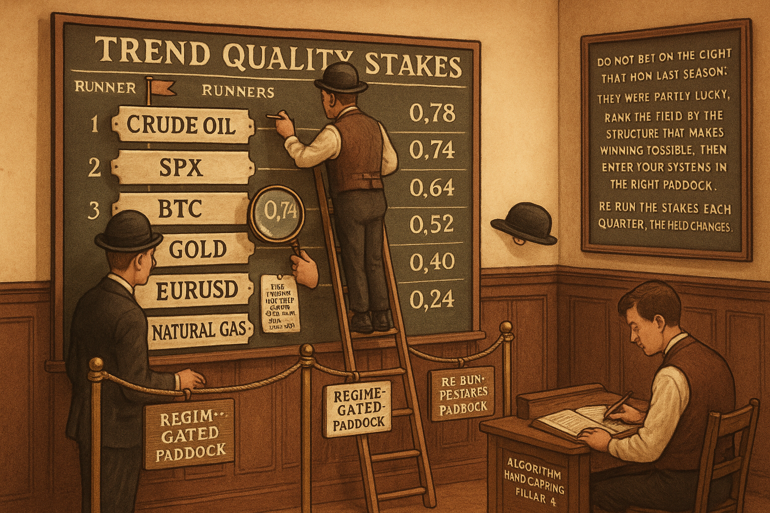
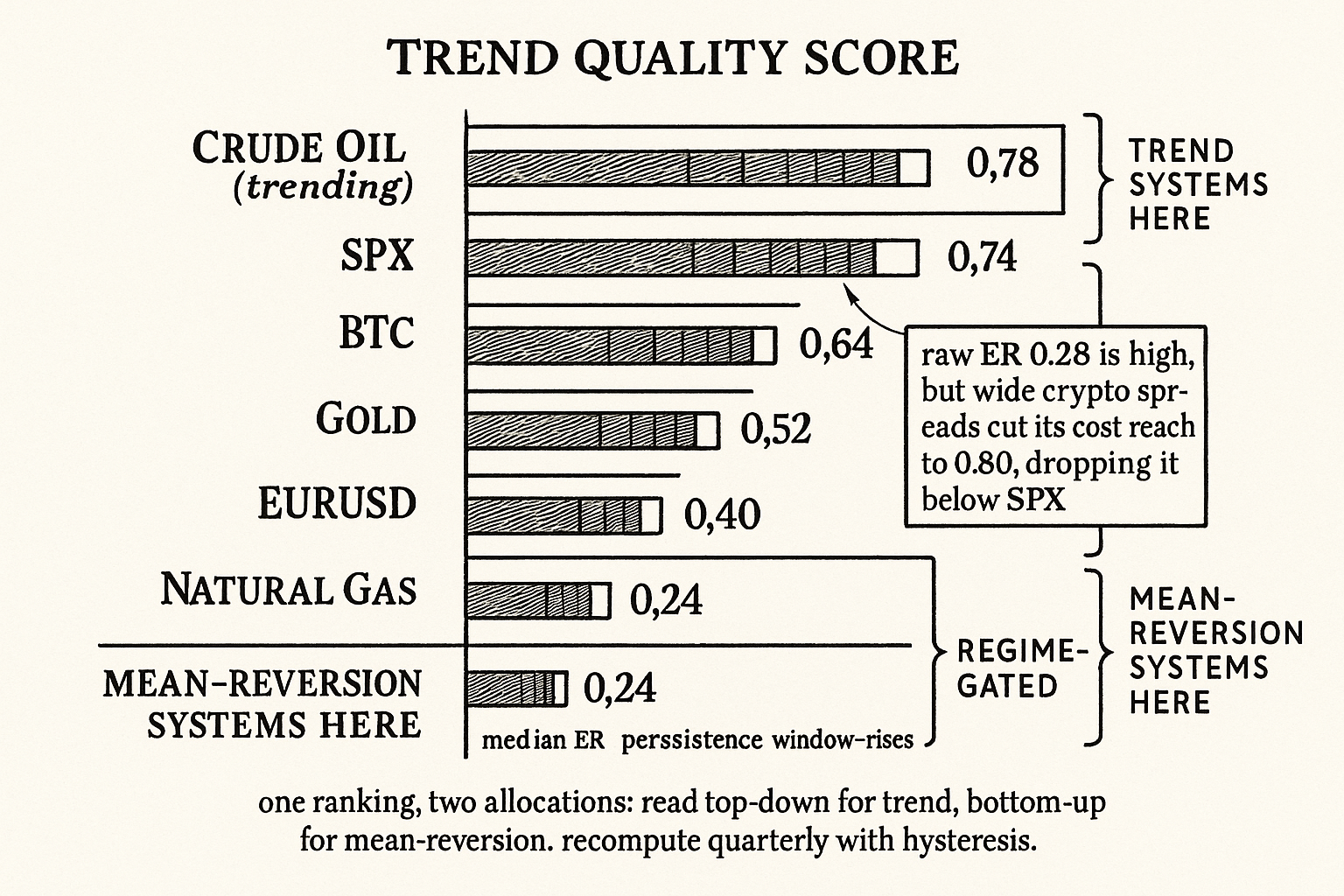
Crude oil (trending regime)	0.34	0.55	yes	0.92	0.78	1
SPX index	0.30	0.50	yes	0.98	0.74	2
BTC	0.28	0.45	yes	0.80	0.64	3
Gold	0.22	0.30	yes	0.95	0.52	4
EURUSD	0.18	0.18	weak	0.97	0.40	5
Natural gas	0.12	0.10	no	0.70	0.24	6

The ranking sorts the universe into a trend-system allocation. The top three (crude in a trending regime, SPX, BTC) are where a trend system should run. The bottom two (EURUSD, natural gas) are where it should not, and where a mean-reversion system should run instead. Gold straddles, which matches its two-mode personality. Note that BTC's high efficiency ratio is partly discounted by its weaker cost reach (wide crypto spreads), which is the cost adjustment doing its job, dropping it below SPX despite a comparable raw efficiency ratio, the same cost-family point the article "Market Personality" made about crypto's 50-to-200-basis-point round trips.

Why ranking beats absolute thresholds

A fixed threshold ("trade trend systems only where the efficiency ratio exceeds 0.30") fails in two directions. In a universe where everything is choppy (an all-FX book), it leaves you with nothing to trade even though some FX crosses are relatively more trend-friendly than others and a trend overlay on the best of them still beats cash. In a universe where everything is trendy (a commodity-heavy book during a macro shock), it tells you to trade everything and gives no basis for choosing the 8 you have capital for. A ranking adapts to the universe: it always identifies the relatively-best trend candidates and the relatively-best mean-reversion candidates, which is the decision you actually face. This is the same reason cross-sectional ranking beats absolute cutoffs in factor work; the relative ordering is more stable than the absolute level.

The ranking also gives you the mean-reversion book for free. Invert it. The bottom of the trend-quality ranking is the top of the mean-reversion-quality ranking, because high noise is exactly what fade and grid systems need, the point the article "Why Grid Systems Need Noise, Not Just Volatility" develops. One ranking, two allocations: trend systems to the top, mean-reversion systems to the bottom.

Rebuild the ranking on a schedule

Trend quality is a structural property, but structures drift, slowly, the way the article "Slow Wandering: The Most Dangerous Type of Market Change" described. A market that ranked first on trend quality in a 3-year supply-shock regime can fall to mid-pack when the shock resolves and the commodity goes back to range-bound seasonality. The discipline is to recompute the ranking on a rolling basis (quarterly is a reasonable cadence) and let allocations follow the ranking, with hysteresis so you are not churning instruments on small rank changes. An instrument has to move several ranks, not one, before you reallocate, because rank noise on a finite sample is real and the small-sample fragility from "Trade-Count Thresholds for Backtest Reliability" applies to the ranking inputs too.

The forward-looking caveat: the ranking predicts trend quality assuming the recent structural regime persists. It is a conditional bet, not a guarantee. A market that ranks high because of a regime that is about to end will disappoint, and there is no way to rank around a regime change you cannot see coming. The ranking reduces selection bias and aligns strategy to structure; it does not see the future, and pretending otherwise is the inductive overreach the article "Induction in Trading: Why Past Patterns Are Always Uncertain" warned about.

Decision summary

Trend-quality rank	Allocation	Rationale
Top tier	Trend, breakout, momentum systems	High median ER, high persistence, reachable after cost
Middle tier	Regime-gated or dual systems	Mixed ER, switch family with the regime
Bottom tier	Mean-reversion, fade, grid systems	High noise is the fuel for these families

The single ranking produces the whole allocation map: trend systems to the top, regime-gated systems to the middle, mean-reversion systems to the bottom, recomputed quarterly with hysteresis.

Visualizing the trend-quality ranking

KEY POINTS

Ranking markets by trend quality beats keeping the 8 best backtest Sharpes from a universe of 40, because the best backtest Sharpes are partly the luckiest (in-sample selection bias). Rank by structure first, confirm with backtest second.
Trend quality combines four components: median efficiency ratio at the trading horizon (use median, not mean, to discount one-off regime spikes), persistence (fraction of time above the trend threshold), window monotonicity (the efficiency ratio should rise with window length for a real trend), and cost-adjusted reach (net move per trade minus round-trip cost).
The composite score weights these roughly 0.4 / 0.3 / 0.1 / 0.2. The weights are arbitrary starting points; the ranking is more robust than the exact weights, which is the property you want.
A worked universe ranks crude (trending) and SPX at the top, BTC third (its high efficiency ratio discounted by wide crypto spreads), gold straddling, EURUSD and natural gas at the bottom.
Ranking beats fixed thresholds because it adapts to the universe: in an all-choppy book it still finds the relatively-best trend candidate; in an all-trendy book it still discriminates among them for limited capital.
The ranking gives the mean-reversion book for free: invert it. The bottom of trend quality is the top of mean-reversion quality, because high noise is fade and grid fuel.
Recompute the ranking quarterly with hysteresis so small rank changes do not churn allocations. Rank noise on finite samples is real; require a move of several ranks before reallocating.
The ranking is a conditional bet that the recent structural regime persists. It reduces selection bias and aligns strategy to structure; it does not predict regime changes, and pretending otherwise is inductive overreach.
The next article, "High Noise Markets Are Mean-Reversion Markets", develops the bottom of this ranking: why the choppy instruments are precisely where fade and reversion systems earn their edge.