4. Market Structure Notes June 1, 2026 9 min

4.2 Efficiency Ratio Explained for Traders

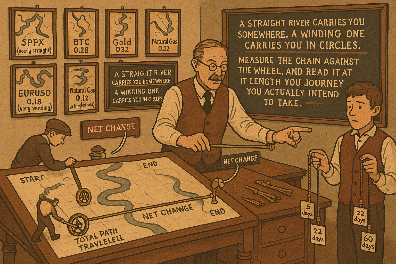
The efficiency ratio is net change over total path, between 0 and 1. It measures how much of a market's motion became direction. Read it at your trading horizon, then pick your strategy family.

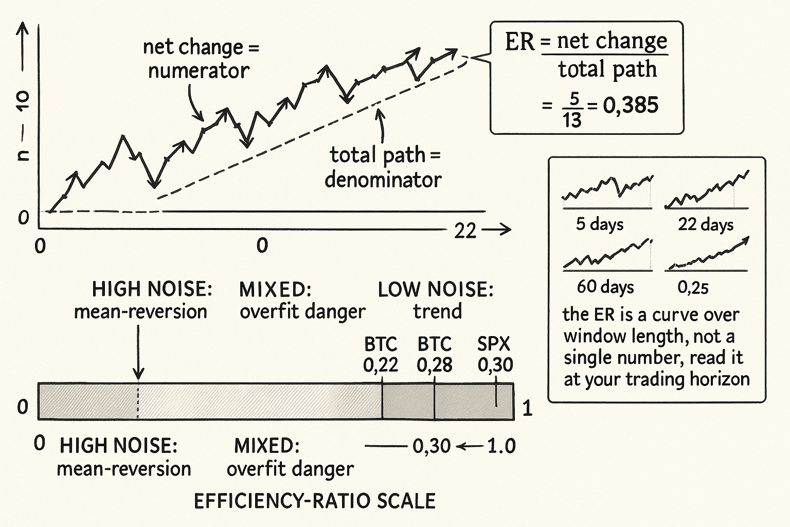
Take a 10-day window of closing prices: 100, 101, 100, 102, 101, 103, 102, 104, 103, 105. The price ended at 105 and started at 100, so the net change is 5 points. Now add up every day's absolute move: from 100 to 101 is 1, 101 to 100 is 1, 100 to 102 is 2, 102 to 101 is 1, 101 to 103 is 2, 103 to 102 is 1, 102 to 104 is 2, 104 to 103 is 1, 103 to 105 is 2. That sums to 13 points of total travel. Divide the net change by the total travel: 5 divided by 13 equals 0.385. That number is the efficiency ratio for this window, and it says the market converted 38.5% of its motion into net direction. The rest, 61.5%, was noise that cancelled out.

The efficiency ratio is the primary tool for measuring the noise the previous article, "Noise Is Not Volatility", isolated. It answers one question with one number between 0 and 1: of all the distance this market travelled, how much actually went somewhere. The article "Market Personality: Why Gold, FX, Crypto, and Equities Need Different Systems" used it to fingerprint instruments; this article is the full mechanics, the window-selection problem, the interpretation thresholds, and the failure modes, so you can compute it correctly and not fool yourself with it.

The formula and what each part means

Two ingredients: net change in the numerator, total path in the denominator.

$$ \text{ER}_W = \frac{|P_t - P_{t-W}|}{\displaystyle\sum_{i=t-W+1}^{t} |P_i - P_{i-1}|} $$

The numerator is the absolute difference between the price now and the price W bars ago. It does not care about the route; it only cares about the two endpoints. The denominator is the sum of the absolute bar-to-bar moves across the whole window, the actual route length. Because the straight-line distance between two points is always less than or equal to the length of any wiggling path between them, the numerator can never exceed the denominator. The ratio is therefore trapped between 0 and 1. A value of 1 means the path was a perfect straight line; every bar moved in the same direction with no backtracking. A value of 0 means the price returned exactly to where it started; all motion cancelled.

Note that the denominator is closely related to the kind of motion an average true range captures, which is why the efficiency ratio is sometimes described as net change divided by summed range. The article "Why ATR Normalization Is More Than a Volatility Trick" used range to scale volatility; the efficiency ratio reuses the same raw material but puts net change on top of it, turning a volatility quantity into a directionality quantity.

The window length is the whole game

The efficiency ratio is not one number; it is a curve indexed by the window W. The same market reads as high-efficiency on one window and low-efficiency on another, and this is not a bug, it is the signal.

Compute the efficiency ratio on EURUSD at three windows. At a 5-day window it might read 0.12 (over a week the price chops and goes nowhere). At a 22-day window it reads around 0.18 (over a month a little net drift survives the chop). At a 60-day window it might read 0.25 (over a quarter a macro lean accumulates). The reading climbs with the window because short-horizon flow is mean-reverting and long-horizon flow carries a slow directional component. Now do the same on a trending commodity: 5-day 0.30, 22-day 0.45, 60-day 0.55. Higher at every window, and rising faster, because the persistence is present even at short horizons.

The practical rule: the efficiency ratio must be computed at the horizon your strategy actually trades. A system that holds positions for two to three weeks should read the efficiency ratio on a window matched to that holding period, not on a 5-day window that reflects microstructure the system never touches. Reading it on the wrong window is the same category of error the article "How to Choose the Right Timeframe for a Strategy" addresses: you measured the wrong horizon's property and concluded something false about the horizon you trade.

A second rule: report the efficiency ratio as a small profile, not a point. Three windows (short, your-horizon, long) tell you whether the market's directionality is concentrated at your horizon or borrowed from a longer one. A market that is efficient only at 60 days but choppy at your 10-day horizon is not a trend market for you, no matter how clean the quarterly chart looks.

Interpretation thresholds, with the usual caveats

The number is continuous, but trading decisions are discrete, so you need thresholds. These are approximate and instrument-dependent; treat them as starting calibrations, not constants.

Below roughly 0.20: high noise. Mean-reversion and fade strategies have their best environment here. Trend systems struggle because the net direction is small relative to the chop they must endure. Most G10 FX sits here at short and medium horizons.

Roughly 0.20 to 0.30: mixed. Neither family has a structural advantage; this is where parameter sensitivity is highest and where most overfitting happens because a system can be tuned to look good on either side. Treat results in this band with the skepticism the article "The Hill, the Spike, and the Cliff: Reading Optimization Surfaces" recommends for fragile peaks.

Above roughly 0.30: low noise, trend-friendly. Breakout and moving-average systems have their structural environment. Sustained equity-index uptrends, commodity supply-shock runs, and crypto breakout regimes live here. The article "Market Personality" put SPX around 0.30 and BTC around 0.28 at a 22-day window, which is why both support multi-week trend frameworks.

These bands are why the efficiency ratio is a strategy-selection tool before it is a signal. You read the regime first and pick the family second, the sequencing the article "Market Personality" insisted on.

A worked cross-market table

Compute the 22-day efficiency ratio across a representative set, the same instruments the personality article fingerprinted, so the numbers tie out.

Instrument	22-day ER (approx)	Read
SPX index	0.30	Trend-friendly, long-bias
BTC	0.28	Trend-friendly in active regimes, regime-variable
Gold	0.22	Mixed, two distinct modes
EURUSD	0.18	High noise, mean-reversion territory
Natural gas	0.12	Very high noise, seasonal

The pattern: equity indices and crypto sit in trend territory, gold straddles, and FX and natural gas sit in chop territory. A trend system deployed across this whole set without reading the column will earn its edge on SPX and BTC and donate it back on natural gas and EURUSD, producing a blended result that looks mediocre and tells you nothing, the exact "run it on everything" trap from "Why Works on All Markets Is Usually a Red Flag".

Using the efficiency ratio as a live filter

The efficiency ratio is not only a research-time classifier; it can gate live signals. The mechanism: compute the rolling efficiency ratio at your horizon and only allow trend entries when it is above your trend threshold, only allow fade entries when it is below your chop threshold. This is the original purpose the indicator was built for, adapting trend speed to noise, and it generalizes to a regime gate on any strategy.

The adaptive moving average it underpins varies its own speed with the efficiency ratio: it scales a smoothing constant so the average moves fast when the efficiency ratio is high (a clean trend worth tracking closely) and slow when the efficiency ratio is low (a chop worth ignoring).

$$ \alpha_t = \big[\, \text{ER}_t \cdot (\alpha_{\text{fast}} - \alpha_{\text{slow}}) + \alpha_{\text{slow}} \,\big]^2 $$

The smoothing constant alpha runs between a fast value (used when the efficiency ratio is near 1) and a slow value (used when the efficiency ratio is near 0). When the market is efficient, alpha is large and the average hugs price; when the market is noisy, alpha shrinks and the average flattens, refusing to chase whipsaws. The squaring sharpens the response so that mid-range efficiency readings still produce a slow average, which is the conservative choice because the mixed band is where false trends live. This is one concrete use; the broader point is that the efficiency ratio can be wired into entry permission, position sizing, or smoothing speed, all driven by the same noise measurement.

Failure modes that will fool you

Four ways the efficiency ratio misleads if you are careless.

Failure 1: gap distortion. A single overnight gap inflates both numerator and denominator but can spike the ratio toward 1 on a short window, falsely signalling a clean trend when the move was one discontinuous jump. Cap or winsorize extreme single-bar moves before computing, or compute on a horizon long enough that one gap does not dominate.

Failure 2: short-window instability. On a 5-day window the ratio is jumpy and the small-sample fragility the article "Trade-Count Thresholds for Backtest Reliability" described applies in full; a single window of five bars is five data points. Do not make regime decisions off a single short-window reading; require persistence across several windows or use a longer horizon.

Failure 3: trend-direction blindness. The numerator uses absolute value, so the efficiency ratio is direction-agnostic. A clean downtrend and a clean uptrend both read high. The efficiency ratio tells you a trend exists, not which way it points; you still need a separate direction input. Pairing it with a slope sign is the standard fix.

Failure 4: regime non-stationarity. The efficiency ratio drifts with the market's personality, which the article "Slow Wandering: The Most Dangerous Type of Market Change" warned moves slowly but inexorably. A threshold calibrated on 2015 data may be miscalibrated by 2025. Recompute the instrument's efficiency-ratio distribution periodically and re-set the thresholds against the current distribution, not a frozen one.

Decision summary

Efficiency ratio at your horizon	Regime	Strategy family	Sizing note
Below 0.20	High noise	Mean-reversion, fade, grid	Scale to volatility, expect many small trades
0.20 to 0.30	Mixed	Neither structurally favored	High overfit risk, demand robustness
Above 0.30	Low noise	Breakout, moving-average, momentum	Scale to volatility, expect few large trades

The table is the operational core: read the ratio at the horizon you trade, map it to the regime, pick the family the regime favors, and only then tune parameters.

Visualizing the efficiency ratio

KEY POINTS

The efficiency ratio is net directional change divided by total absolute path length over a window, trapped between 0 and 1. It measures what fraction of a market's motion converted into net direction; the rest is noise.
Worked example: a 10-day window ending 5 points higher with 13 points of total travel reads 5 over 13, equal to 0.385. The market converted 38.5% of its motion into direction.
The window length is not a detail; it is the signal. The same market reads choppy on a 5-day window and efficient on a 60-day window. Compute the ratio at the horizon your strategy actually trades.
Report a small profile (short, your-horizon, long) rather than a point. A market efficient only at long horizons but choppy at your horizon is not a trend market for you.
Threshold calibration: below 0.20 is high noise (mean-reversion territory), 0.20 to 0.30 is mixed (highest overfit risk), above 0.30 is low noise (trend territory). Approximate and instrument-dependent.
Cross-market 22-day readings tie out with the personality fingerprint: SPX 0.30, BTC 0.28, Gold 0.22, EURUSD 0.18, natural gas 0.12. Equities and crypto sit in trend territory, FX and natural gas in chop.
The efficiency ratio is a strategy-selection tool before it is a signal. Read the regime first, pick the family second, tune parameters last.
It can gate live signals and drive an adaptive moving average whose smoothing constant scales with the ratio: fast average in efficient markets, flat average in noisy ones, with squaring to stay conservative in the mixed band.
Four failure modes: single-gap distortion (winsorize), short-window instability (require persistence), direction-blindness (the absolute value hides trend direction, pair with slope sign), and threshold non-stationarity (recompute the distribution periodically).
The next article, "How to Rank Markets by Trend Quality", turns the efficiency ratio from a per-market reading into a cross-market ranking system for allocating strategies to instruments.