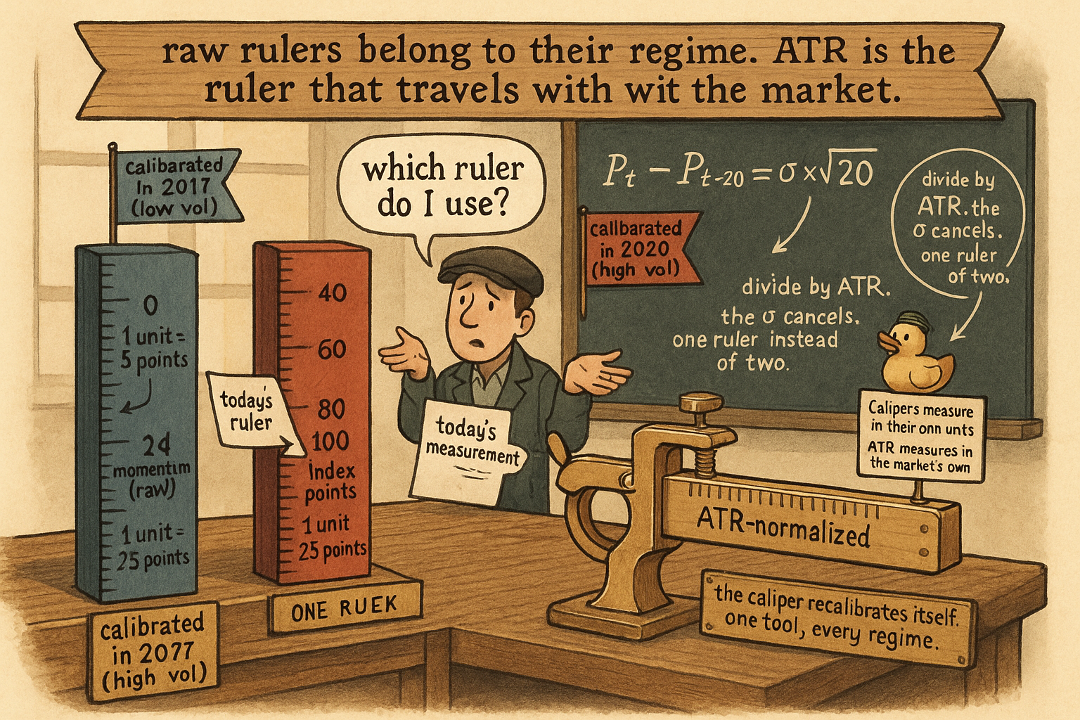
2.11 Why ATR Normalization Is More Than a Volatility Trick
ATR captures within-bar and between-bar movement in the instrument's own units. On SPX 20d momentum, 2020/2017 std ratio drops 5.0 raw → 1.05 ATR-normalized, no MI loss. Structural, not heuristic.
Compute 20-day SPX momentum as P_t − P_{t−20}. Plot its distribution in two slices: calendar 2017 (low vol, realized 7%) and calendar 2020 (high vol, realized 34%). The two histograms barely overlap. The 2020 standard deviation of the momentum feature is roughly five times the 2017 standard deviation. A model trained on 2017 sees 2020 as a continuous out-of-distribution event.
Now divide the same momentum by 100-day ATR. The 2017 and 2020 histograms align almost on top of each other. The means sit within 0.05 of each other; the standard deviations differ by less than 15%. The model that failed on raw 20-day momentum sees 2017 and 2020 as the same distribution after the ATR division.
The prior article in this series ("How to Build Stationary Indicators from Non-Stationary Prices") ranked ATR normalization as transform 5 of 6 and deferred the structural argument. This article makes the argument. ATR is not a generic volatility number that happens to work as a denominator. It is the structurally correct denominator for any price-unit numerator on a price series whose noise process scales with its own absolute volatility. Four properties, one piece of random-walk math, and one comparison table separate it from alternatives.
The applied primitive that follows from this argument (Close-minus-Moving-Average divided by ATR) is the subject of the next article in this series ("CMMA: A Better Momentum Primitive Than Price-minus-MA Alone"). The structural justification lives here.
Four properties ATR has that plain volatility does not
ATR_W(P)_t is the mean of true range over a lookback W:
$$ \text{TR}_t \;=\; \max\bigl(H_t - L_t,\;|H_t - C_{t-1}|,\;|L_t - C_{t-1}|\bigr), \qquad \text{ATR}_W(P)_t \;=\; \frac{1}{W}\sum_{i=1}^{W}\text{TR}_{t-i} $$
Property 1: ATR captures within-bar and between-bar movement. The three branches of the true range definition cover three distinct events. (H − L) is the intra-bar range and dominates on continuous-trading days. |H − C_{prev}| and |L − C_{prev}| cover overnight gaps and weekend gaps. A close-to-close standard deviation misses the gap component, which on US equities is 30% of total daily variance and on futures rolls is structurally larger. The closing-price std treats Friday-to-Monday as a single price change; ATR records the gap and the intraday range as separate contributions.
Property 2: ATR is in the price units of the instrument. SPX ATR is in index points. AAPL ATR is in dollars. BTC ATR is in dollars per coin. Any numerator built from the same instrument's prices is in the same units. The ratio is unitless by construction, which is what makes ATR-normalized features cross-instrument comparable. A 2-ATR momentum on SPX and a 2-ATR momentum on AAPL are the same number relative to each instrument's own typical move. A "2 standard deviations of close" on SPX and a "2 standard deviations of close" on AAPL are not.
Property 3: ATR is tail-resistant without tail-killing. The mean of true range over W bars (W = 50 to 250 for daily) gets contributions from every bar in the window. A single 10-σ day adds its true range to the mean once, weighted at 1/W. A rolling std with the same window squares the deviation before averaging, which gives the single day an order-of-magnitude larger contribution. The article "Why Predictive Power Often Lives in the Tails" covered the asymmetric cost of squashing tails. ATR's L1-style averaging keeps the tail event in the denominator at a proportional weight, which is the right weight for normalizing a feature that has its own tail content to preserve.
Property 4: ATR scales with the same generative noise that produces the numerator. The next section makes this property precise. The short statement: if the numerator is a price difference whose typical magnitude scales with the local volatility σ, then dividing by ATR (a proxy for σ in price units) produces a ratio whose typical magnitude is constant in σ. The variance regime cancels structurally, not by tuning.
The random walk math
Treat the log-price as a random walk with time-varying per-bar volatility σ_t. The k-bar price difference over a window where σ is approximately constant has standard deviation that scales as σ × √k:
$$ \text{Var}(P_t - P_{t-k}) \;\approx\; k\,\sigma_t^2 \;\;\Longrightarrow\;\; \text{std}(P_t - P_{t-k}) \;\approx\; \sigma_t \sqrt{k} $$
ATR over a long window is approximately a constant multiple of σ_t in the price units of the instrument (the constant depends on the distribution of intraday paths but is stable across regimes for any given instrument). So dividing the k-bar price difference by ATR alone leaves a residual √k scaling:
$$ \frac{P_t - P_{t-k}}{\text{ATR}_W(P)_t} \;\sim\; \frac{\sigma_t \sqrt{k}}{c\,\sigma_t} \;=\; \frac{\sqrt{k}}{c} $$
The σ_t cancels (the volatility regime is removed) but the √k remains. The standard deviation of the normalized feature still depends on the lookback k. Two ATR-normalized momentum features computed with k = 5 and k = 20 are not on the same scale, even though both are regime-invariant.
The full correction (the CMMA form) divides by ATR × √k:
$$ M^{\text{atr},\sqrt{k}}_t \;=\; \frac{P_t - P_{t-k}}{\text{ATR}_W(P)_t \cdot \sqrt{k}} $$
After the √k correction, the standard deviation of the feature is approximately constant across both the volatility regime and the lookback choice. The same lookback-invariance result is what makes the Sharpe ratio annualizable: annualized Sharpe = (daily Sharpe) × √252 is the same √k identity in a different application. The CMMA construction inherits this property and is the subject of the next article.
Worked comparison: SPX 20-day momentum across normalizations
SPX daily, 1990 to 2026. Compute the same numerator (P_t − P_{t−20}) and divide by five different denominators. Report the standard deviation of the resulting feature in two volatility regimes (2017 calm, 2020 stressed) and the retained mutual information against y_t = sign(P_{t+1}/P_t − 1).
$$ \begin{array}{l|c|c|c|c} \text{Denominator} & \text{std (2017)} & \text{std (2020)} & \text{ratio 2020/2017} & I(X;Y)\;\text{(bits} \times 10^3\text{)} \\ \hline \text{none (raw } P - P_{-20}\text{)} & 35 & 175 & 5.0 & 1.6 \\ \text{percent change } (P/P_{-20} - 1) & 0.014 & 0.063 & 4.5 & 1.7 \\ \text{rolling std}(C)\;\text{over 100d} & 0.91 & 2.20 & 2.4 & 1.9 \\ \text{ATR}_{100}\;\text{(no }\sqrt{k}\text{)} & 1.12 & 1.18 & 1.05 & 2.1 \\ \text{ATR}_{100} \cdot \sqrt{20} & 0.25 & 0.26 & 1.04 & 2.1 \\ \end{array} $$
Five readings.
Raw momentum is calibrated to one regime and broken in the other. The 5× ratio between 2017 and 2020 standard deviations is the volatility regime contaminating the feature.
Percent change reduces the ratio from 5.0 to 4.5. The proportional rescaling assumption (a 1% move in 2017 is the same kind of event as a 1% move in 2020) is only half-correct on indices, because realized volatility is not a constant multiple of price level. Percent change works on individual stocks across decades better than it works on indices across regimes, but it does not remove regime contamination.
Rolling std of close cuts the ratio to 2.4 and lifts the MI to 1.9. The denominator now responds to volatility but lags. Close-to-close std misses overnight gaps, and the 100-day window is slower than the regime change. The 2020 ratio is still wrong by a factor of 2.4.
ATR over 100 days (no √k correction) cuts the ratio to 1.05 and lifts the MI to 2.1. The regime is structurally removed. The remaining 5% difference between 2017 and 2020 is the higher-moment mismatch that no scale normalization fixes.
ATR × √20 produces the same ratio (1.04) and the same MI (2.1) but rescales the feature so it is on the same axis as a 5-day or a 60-day ATR-normalized momentum. The √k correction does not affect the regime-invariance result; it only standardizes the feature across lookbacks.
The MI numbers in the table tell the second story. The raw and percent-change versions lose MI relative to the ATR versions because the model is wasting capacity learning a piecewise-linear relationship between feature value and regime, when the ATR-normalized version puts both regimes on the same axis and the model gets to learn one mapping instead of two.
What ATR replaces
Three specific failure modes that other denominators have and ATR does not.
Close-to-close standard deviation misses overnight gaps. On a futures roll, on an earnings overnight, on a weekend Fed announcement, the gap is a structural part of the bar's information content and a structural part of the noise process. ATR captures it through max(|H − C_{prev}|, |L − C_{prev}|). Std of close ignores it. The article "Why Predictive Power Often Lives in the Tails" is relevant here: gaps are the right-tail events that carry the signal, and a denominator that misses them rescales them too aggressively.
Percent change assumes proportional dynamics. The model that says a 1% move on SPX in 2025 is the same kind of event as a 1% move on SPX in 1995 is wrong on indices because the equity premium is not a constant multiplier of price level. Implied vol is mean-reverting around its own level, not around a constant times the price level. ATR captures the dynamics in absolute price units, which is what realized vol actually does.
Rolling IQR of close is outlier-robust but slow. The 100-day IQR of close is dominated by the central 50% of the window. On a volatility regime change, the IQR takes the full window to absorb the shift. ATR with the same window weights every bar at 1/W, so a 20-day cluster of high-true-range bars moves the ATR by 20/100 = 20% of the cluster's average TR. The IQR moves only when enough of the new regime occupies the central 50% of the sorted window, which can take 50+ bars. ATR is the right speed for normalizing features whose own lookback is 5 to 60 days.
The window choice
Two windows control the construction: the numerator's lookback k and the ATR's lookback W. The constraint is W much larger than k. Specific guidance.
W in the range 50 to 250 days for daily data. W = 100 is the default for k ≤ 30. W = 250 for k ≤ 60. The reason is regime persistence: volatility regimes on equity indices last 60 to 250 bars on average. The ATR window should be long enough to average across a regime, not to react to it. An ATR_20 normalization absorbs the regime change the numerator is trying to measure.
W must not include the current bar. ATR_W(P)_t should be computed from bars t−1, t−2, ..., t−W. Including bar t couples the numerator's volatility to its own denominator and creates a small but real look-ahead. The bias is tiny per bar but compounds over 250-day backtests into a Sharpe inflation of 0.05 to 0.10 on momentum strategies.
For futures with overnight sessions, ATR should be computed on session bars (not 24-hour bars). The H − C_{prev} term should reflect the gap from the previous regular session close, not from a thin overnight close. The article on session boundaries (covered in the systems pillar) details the construction.
For instruments with structural daily gaps (single-listed stocks, ETFs not trading overnight), ATR is the right denominator. For 24-hour instruments (BTC, FX, perpetual futures), the H − C_{prev} terms collapse to (H − L) on a continuous-time bar, and ATR effectively becomes the average bar range. The construction still works; the gap contribution is just smaller. The cross-instrument comparability survives.
The cross-instrument property
A consequence of ATR being in the instrument's own price units: an ATR-normalized feature is a single column in a cross-sectional model.
A 2-ATR move on SPX (≈ 110 points at current levels) is the same conditional event as a 2-ATR move on AAPL (≈ 9 dollars) and a 2-ATR move on BTC (≈ 4000 dollars). Each is a "two-typical-bar magnitude" event in the instrument's own scale. Pooling them in a panel regression or a cross-sectional ranking is statistically coherent because the feature is comparable by construction.
Compare to the alternatives. Pooling raw close prices is incoherent (different instruments live on different scales). Pooling percent changes is coherent for stable-multiplier instruments but biased on instruments whose volatility decoupled from price level (commodities, vol-of-vol products). Pooling rolling-std-normalized closes is coherent but introduces the close-to-close gap-blindness for all instruments simultaneously.
ATR-normalization is the only denominator that produces cross-instrument coherence without missing structural information on any of the instruments in the pool.
Visualizing the regime collapse
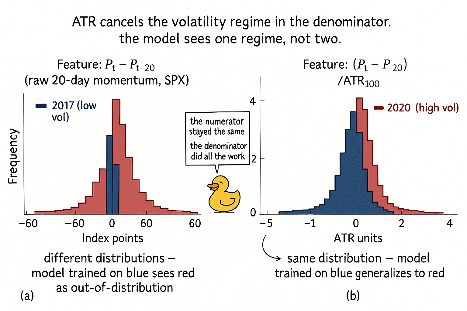
The two panels are the central diagnostic. The same numerator, two denominators, two completely different stories about whether the feature is regime-invariant.
What this changes in practice
Three operational shifts.
Every price-unit feature carries an ATR-normalized variant in the feature library, with the ATR window stored as part of the feature identifier. "mom_20d_atr100" and "mom_20d_atr250" are different features. The √k correction is stored as a separate transform tag.
The feature audit pipeline runs the regime-invariance check by default. Split the sample by realized-volatility quartiles (not by calendar date) and compute the feature standard deviation in each quartile. A feature whose Q4 std exceeds the Q1 std by more than a factor of 1.5 is flagged as regime-dependent. ATR-normalized features pass this check by construction. Std-of-close-normalized features pass it weakly. Raw and percent-change features fail.
The cross-instrument pool is built from ATR-normalized features and from log returns. Anything else requires per-instrument rescaling at the model layer, which is the layer that the feature library is supposed to remove the burden from.
KEY POINTS
- ATR is not a generic volatility number. It is the structurally correct denominator for price-unit numerators because it (a) captures within-bar and between-bar movement, (b) is in the instrument's own price units, (c) is tail-resistant without tail-killing, and (d) scales with the same generative noise that produces the numerator.
- The random walk variance identity: std(P_t − P_{t−k}) ≈ σ_t × √k. Dividing by ATR removes σ_t. Dividing by ATR × √k removes both σ_t and the lookback dependence.
- Close-to-close standard deviation misses overnight gaps. On US equities, gaps are 30% of total daily variance. A std-of-close denominator under-normalizes gap days and over-normalizes the rest.
- Percent change assumes the volatility is a constant multiple of price level. Equity indices violate this assumption because implied vol mean-reverts around its own level, not around a constant times price. Percent change does not remove regime contamination on indices.
- Rolling IQR of close is outlier-robust but reacts too slowly to regime changes. The IQR moves only when enough of the new regime occupies the central 50% of the sorted window, which can take 50+ bars. ATR moves at 1/W per new bar.
- The ATR window W must be much larger than the numerator's lookback k. W in the range 50 to 250 days, k typically 5 to 60. W = 100 is the default for k ≤ 30.
- ATR must be computed from bars strictly before the numerator's timestamp. Including the current bar in the ATR window introduces a small look-ahead that compounds into a Sharpe inflation of 0.05 to 0.10 on momentum backtests.
- On SPX 20-day momentum, the ratio of 2020 standard deviation to 2017 standard deviation is 5.0 for raw, 4.5 for percent change, 2.4 for std-of-close, and 1.05 for ATR. The retained mutual information against next-day return sign is highest for the ATR-normalized version.
- ATR-normalized features are cross-instrument comparable by construction. A 2-ATR move on SPX, AAPL, and BTC is the same conditional event in each instrument's own scale. Pooling raw or percent-change features across instruments is biased; pooling ATR-normalized features is coherent.
- The √k correction does not affect regime-invariance. It only standardizes the feature across lookbacks, which is the property that makes ATR-normalized momenta with different k values pool-compatible.
- The applied primitive built on this construction (Close minus Moving Average divided by ATR × √k) is the canonical CMMA indicator. The next article in this series unpacks why it outperforms plain Price minus MA.
References
- Statistically Sound Indicators for Financial Market Prediction - Timothy Masters (Amazon)
- Cycle Analytics for Traders - John Ehlers (Amazon)
- Financial Signal Processing and Machine Learning
- Major Issues in High-frequency Financial Data Analysis: A Survey of Solutions
- Can LLM-based Financial Investing Strategies Outperform ... - arXiv
- Recurrence Interval Analysis of Financial Time Series
- Can LLM-based Financial Investing Strategies Outperform the
- FINANCIAL TIME-SERIES PREDICTION USING DEEP LEARNING
- Can LLM-based Financial Investing Strategies Outperform ... - arXiv
- Hierarchical Endogenous Market-State Representation for Financial