2.6 Why Predictive Power Often Lives in the Tails
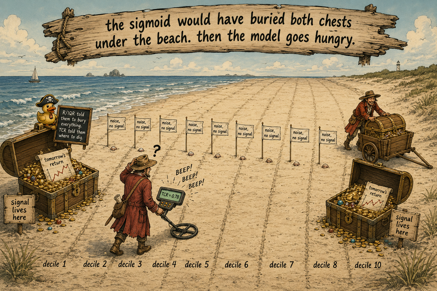
R/IQR detects stretched distributions but says nothing about whether the stretch carries the signal. On market data the stretch usually carries it. The Tail Concentration Ratio splits per-decile mutual information and tells you whether the tails are noise to squash or signal to preserve.
You build a 20-day ATR-normalized momentum on SPX. R/IQR comes back at 11. The prior article in this series ("Range/IQR: A Simple Test for Indicator Tail Problems") gave you the band: tail-dominated, apply a tail-taming transform. You pass it through a z-scored sigmoid. R/IQR drops to 2.0. The loss function is now safe from single-day leverage.
You refit and the AUC drops from 0.518 to 0.506. The sigmoid did not just tame the tails. It compressed the only part of the feature space where the model was finding any signal.
This article is the counter-weight to the prior three. Tail diagnostics tell you the indicator has a stretched distribution. They do not tell you whether the stretch carries information. On real market data the stretch usually does, and the default "every heavy-tailed feature gets a sigmoid" pipeline is throwing the signal out with the tail noise.
Why markets have signal in the tails
Three structural reasons, none of them controversial once stated.
Markets price information through trades. Days with small moves carry no event. Days with large moves carry concentrated information: an earnings surprise, a Fed decision, a liquidity vacuum, a forced unwind. The right tail of the return distribution is where the news lives. A model that wants to learn anything about event-conditional outcomes needs to keep tail magnitudes distinguishable from each other, not collapsed into a single saturated value.
Volatility clusters. A 3σ day on SPX is followed by elevated realized volatility for ten to forty bars on average. A 1σ day is followed by a regime indistinguishable from the long-run average. The conditional distribution of tomorrow's realized volatility given today's |return| is a steep function in the tails and a flat function in the body. If your indicator preserves the body and saturates the tails, you have erased the part of the input that predicts tomorrow's volatility.
Reversals and continuations are tail-conditional. The mean-reversion edge in equity indices sits at the extreme momentum quantiles. The conditional expectation E[r_{t+1} | M_t] is approximately constant across the central 80% of M_t and bends sharply in the top and bottom deciles. A model trained on sigmoid-compressed momentum cannot resolve where in the tail the observation sat, so it cannot price the reversal.
Volume, order-flow, and dispersion features are heavier-tailed than returns, and their predictive content concentrates further into the upper tail. A typical volume day predicts nothing. A 4σ volume day is informative about institutional positioning, information leakage, or a regime break in progress.
The decile decomposition
Mutual information against the target decomposes by quantile bin. Sort X into K equal-frequency bins (K = 10 is the standard daily-frequency choice). Let p_k be the probability of bin k, which is 1/K by construction:
The total MI is the average of K KL divergences, one per decile. For a feature whose signal is uniform across the distribution, each decile contributes equally. For a feature whose signal lives in the tails, the first and Kth deciles dominate and the central deciles contribute near zero.
The Tail Concentration Ratio is the per-decile readout:
For K = 10 a uniformly-informative feature scores TCR ≈ 0.2, since the two extreme deciles are 2 out of 10 equal contributions. TCR ≈ 0.5 means the two tail deciles match the other eight combined. TCR above 0.6 is tail-dominated signal. TCR above 0.8 is "the body is noise."
A Gaussian-noise control should score TCR ≈ 0.2 with total MI near the sampling floor. A control that scores higher TCR with non-trivial total MI is data-snooped, not signal.
Worked example: SPX features by decile
SPX daily, 1990 to 2026, target y_t = sign(P_{t+1}/P_t - 1). Five candidate features split into 10 deciles. Per-decile KL divergences computed against the marginal sign distribution.
Four readings.
Realized volatility carries 78% of its predictive content in the two extreme deciles. A sigmoid through realized vol would compress the 4σ vol days into a flat upper saturation and destroy the part of the feature that was carrying the signal. The right transform for high-TCR realized vol is no transform on the magnitude axis. The R/IQR is high because the signal makes it high, not because the construction is broken.
20-day ATR-normalized momentum scores TCR = 0.64. A sigmoid here erases the mean-reversion edge that lives in the extreme momentum bins, which is the result that opened the article. A rank transform erases it equally hard, since rank discards all magnitude information and the magnitude is exactly what separates the 90th-percentile momentum from the 99th. The right transform is winsorization at 99.5%, which clips the data errors and the one-in-a-decade observations while leaving the rest of the tail gradient intact.
5-day ATR-normalized momentum scores TCR = 0.41. The signal is mixed: some lives in the tails, some in the body. A mild fourth-root or a sigmoid with a wide scale parameter preserves some tail gradient while reducing the loss-function leverage. The transform-choice trade is real and depends on the body-versus-tail split.
Stochastic K(14) scores TCR = 0.22 and R/IQR = 2.0. Body-dominated signal, bounded distribution by construction. No transform is needed and no transform would help. The few features in this category are the ones where the conventional preprocessing advice causes no harm.
The Gaussian control scores TCR = 0.19 and MI = 0.0001. The TCR is at the sampling floor and the MI is at the noise floor. Neither number says anything about predictive content because there is none.
The transform-choice decision matrix
R/IQR tells you the indicator has tail extension. TCR tells you whether the tail extension carries the signal. The two together determine the transform.
R/IQR | TCR | Transform | Reason |
|---|---|---|---|
Below 3 | any | none | bounded already |
Above 5 | Below 0.3 | sigmoid or rank | tails are noise, body holds signal |
Above 5 | 0.3 to 0.6 | fourth-root or wide-scale sigmoid | preserve partial tail gradient |
Above 5 | Above 0.6 | winsorize at 99.5%, or feed raw to trees | tails carry signal, do not squash |
The default of "every heavy-tailed feature gets a sigmoid" is wrong for any feature with TCR above 0.5. The default for high-TCR features is to leave the magnitude intact, or to clip at a percentile far enough out that only data errors get removed.
The percentile choice inside winsorization matters more than the winsorization-versus-sigmoid choice. Clipping at 99.5% on SPX returns removes Black Monday and COVID Monday and three other days, which is a fraction of a percent of the loss-function leverage and approximately zero of the predictive content of the central tail mass. Clipping at 95% removes 450 days, which is 60% of the predictive content of a high-TCR feature.
Why trees do not save you
The common rebuttal: tree-based models are invariant to monotonic transforms, so the transform choice does not matter for XGBoost or LightGBM. The statement is half true and the missing half is the operational one.
Tree splits pick a threshold in the feature's native units. If the feature is sigmoid-bounded, the available thresholds live on [0, 1] and the resolution near the saturated ends collapses. Two observations with raw values M^atr = 4 and M^atr = 6 both pass through the sigmoid to roughly 0.982 and 0.998. The tree's split-finding algorithm sees the gain from a threshold at 0.990 as the difference between two observations both rounded to the third decimal. Floating-point arithmetic preserves the distinction. The gain estimator's variance from finite training data does not. The split between 0.982 and 0.998 sits below the gain noise floor and the tree picks a different split, in the body, where the gain is larger by sampling alone.
The practical statement: for tree models, the transform that preserves tail magnitudes (no transform, or winsorization at 99.5%) keeps more usable tail resolution than the transform that bounds them (sigmoid). The TCR diagnostic applies to trees, gradient-boosted ensembles, and linear models alike.
Visualizing where the signal lives
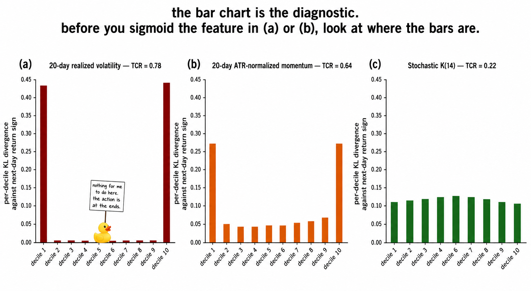
The three panels are the central diagnostic. R/IQR alone would push (a) and (b) into the same "apply sigmoid" bucket. The decile decomposition splits them: (a) cannot afford to lose its tails, (b) can afford to lose a little, (c) has nothing in the tails to lose.
What this changes in practice
Three operational shifts.
The transform pipeline runs in this order: diagnose with R/IQR, diagnose with TCR, then choose the transform. Skipping the TCR step means defaulting to sigmoid on every heavy-tailed feature, which costs roughly the AUC drop from 0.518 to 0.506 in the opening example. The cost compounds across a research portfolio of features because the same default is applied to all of them.
Winsorization at 99.5% is a real option, not a fallback. The 0.5% you clip is data errors plus three days per decade. The 99.5% you keep retains the tail gradient that high-TCR features need. The choice between winsorization and sigmoid is not a matter of preference. It is determined by the TCR.
The transform choice belongs to the feature definition. Two indicators with the same raw construction and different transforms are different features. Log them separately. The R/IQR scores them. The TCR scores them. The transform that maximizes the in-sample MI is overfitting on the diagnostic. Set the transform from the structural reading (where does the signal live in the distribution), not from the in-sample MI lift after each candidate transform.
KEY POINTS
- Tail diagnostics like R/IQR detect stretched distributions but do not say whether the stretch carries information. On market data the stretch typically does.
- Three structural reasons signal lives in market tails: information arrives through large moves, volatility clusters conditional on tail magnitudes, and reversal/continuation edges live in extreme quantiles of momentum and dispersion features.
- The Tail Concentration Ratio (TCR) is the per-decile readout. Sort X into 10 equal-frequency bins, compute per-decile KL divergence against the target, take the share of the total contributed by the two extreme bins.
- TCR around 0.2 is uniform signal across the distribution. TCR above 0.6 is tail-dominated. TCR above 0.8 means the body is noise.
- The transform decision is determined by R/IQR crossed with TCR: bounded features need nothing, high-R/IQR low-TCR features take a sigmoid or rank, high-R/IQR high-TCR features take winsorization at 99.5% or are fed raw into a tree model.
- Sigmoid on a high-TCR feature compresses the tails that carried the signal. The AUC cost is typically 0.01 to 0.02 per feature, which compounds across a research portfolio.
- The percentile choice inside winsorization matters more than the winsorization-versus-sigmoid choice. Clipping at 99.5% removes data errors and a few decade-scale events. Clipping at 95% removes the meaningful tail mass.
- Tree models are not invariant to tail-bounding transforms in practice. Sigmoid-saturated regions collapse the achievable split resolution at the tails, and the tree picks a body split instead by sampling-noise leverage.
- The transform belongs to the feature definition, not to a free knob optimized on the backtest. The R/IQR and TCR fix it before any model sees the data.
- High R/IQR is not by itself a defect. A diagnostic that says "the feature has tails" without saying "the tails are noise" is incomplete.
References
- Statistically Sound Indicators for Financial Market Prediction - Timothy Masters (Amazon)
- Cycle Analytics for Traders - John Ehlers (Amazon)
- Recurrence Interval Analysis of Financial Time Series
- Financial Signal Processing and Machine Learning - Wiley
- Statistical properties of bibliometric indicators: Research group
- Order book characteristics and future price volatility:
- FINANCIAL TIME-SERIES PREDICTION USING DEEP LEARNING
- Multi-scale periodic analysis of financial indexes for quantitative
- Dark Trading at the Midpoint: Pricing Rules, Order Flow, and High
- Hierarchical Endogenous Market-State Representation for Financial