2.5 Range/IQR: A Simple Test for Indicator Tail Problems
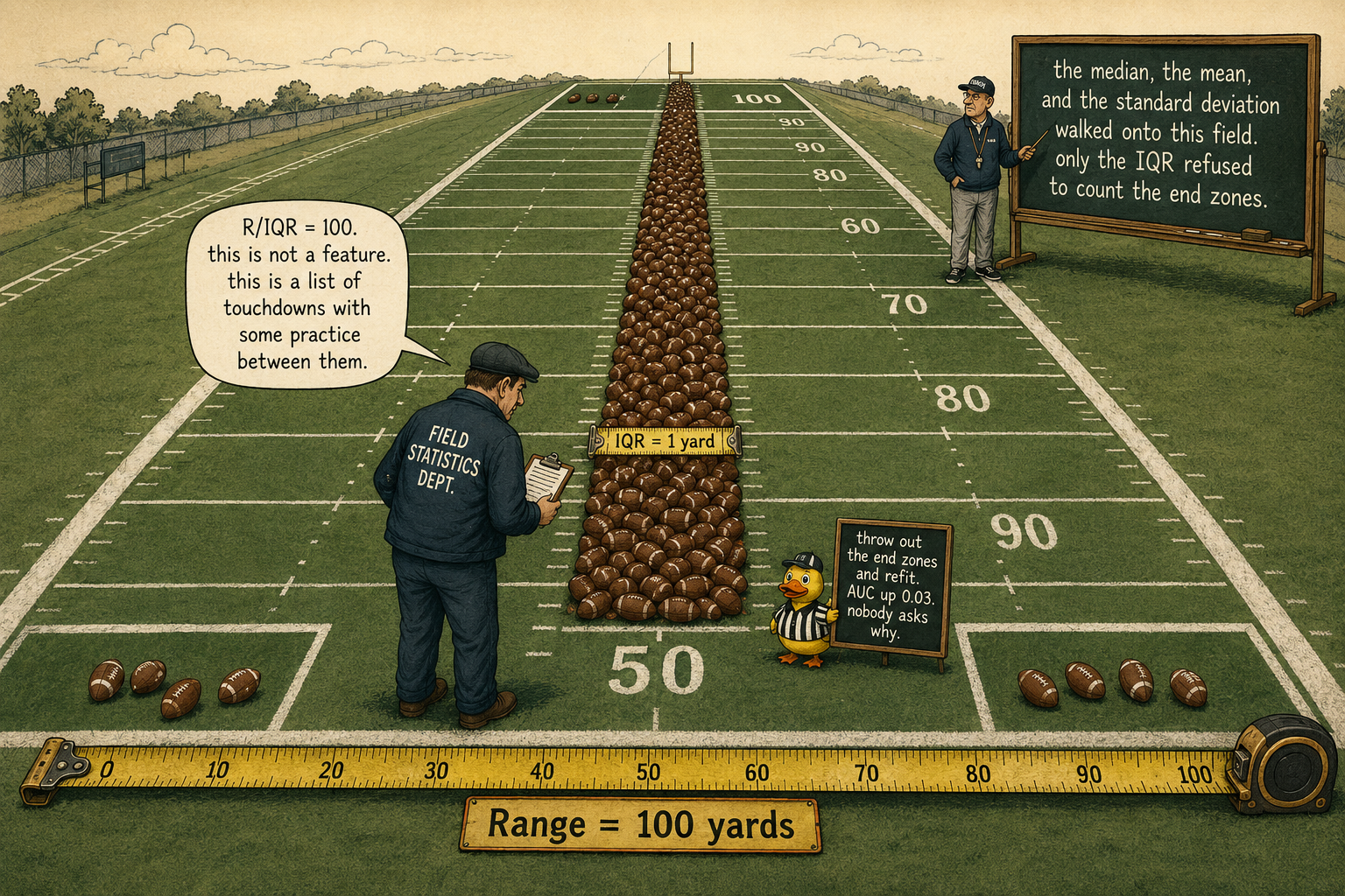
R/IQR is the ratio of total range to interquartile range. The denominator is anchored to the body of the distribution. The numerator follows the tails. The ratio is the only honest tail measurement on data where the standard deviation is already contaminated by the tails it is supposed to describe.
You compute daily returns on SPX from 1928 to 2026. The histogram looks like a bell with a few far-flung dots. You fit a logistic model, get AUC 0.512. You drop the largest 0.1% of observations as "obvious outliers," refit, and the AUC jumps to 0.541. You did not just clean noise. You amputated nine days that carried more than a tenth of the loss-function leverage in the dataset, and you have no diagnostic that flagged the amputation before you trained the model twice and compared the numbers.
R/IQR is the diagnostic. One ratio. Five seconds of computation. It tells you whether your indicator is a smooth feature with a few stragglers or a list of crashes with some noise wrapped around them.
What the ratio measures
The Range-over-IQR ratio is:
The numerator is the full range. The denominator is the interquartile range, the width of the central 50% of the data. The ratio asks how many "central-half widths" you have to stack to span the extremes.
For a uniform distribution the answer is exactly 2: the range is 1.0, the IQR is 0.5. For a Gaussian, the expected maximum of N draws scales with the square root of log N, so the ratio drifts upward with sample size:
On a daily series of 9000 bars (about 35 years), the Gaussian baseline is around 6.3. On 10-minute bars over the same window (about 250,000 bars), it sits closer to 7.4. On a 200-bar window it drops to 4.8. The diagnostic value comes from comparing your indicator's R/IQR to this baseline. Anything noticeably above is heavier-tailed than a Gaussian with the same sample size. Daily SPX returns sit around 30. That is not heavy-tailed in the polite sense. The IQR is the wrong scale for the data.
Why this ratio and not the standard deviation
The natural first try at a tail diagnostic is the standardized range: max minus min, divided by the standard deviation. The standard deviation contains the tails inside its own computation. Squaring the residuals before summing makes sigma scale linearly with the extreme observations. As the tails get heavier, both numerator and denominator grow, and the standardized range moves slowly. A 20σ event raises sigma enough that the ratio barely flinches.
Kurtosis has the same problem with worse leverage. The fourth moment is dominated by single observations on heavy-tailed data. You compute kurtosis on SPX returns, get a number around 24, and that number is mostly 1987 squared a few times over.
Order statistics fix both problems. Q25 and Q75 are positions in the sorted data, not weighted sums. By construction they ignore everything outside the central 50%. Adding a 100σ event to the sample changes the IQR by zero. So the denominator stays anchored to the body of the distribution while the numerator measures how far the tails reach. The ratio is a clean measurement of "tail extent relative to body width," with no contamination of the body measurement by the tails.
This is the same logic that makes the median preferred over the mean on dirty data. Order statistics carry less information than moments under clean conditions, but they refuse to be hijacked by single observations under bad conditions. On real market data the bad conditions are the operating regime.
Worked example: SPX, four candidates, four diagnostics
SPX daily, 1990 to 2026, 9100 bars. Four candidate features built from the same underlying price. R/IQR, the rolling-252-day mean drift, the kurtosis, and the mutual information with the sign of next-day return all computed on each. The Gaussian baseline R/IQR for N = 9100 is 6.3, included for reference.
Four readings.
Raw close scores R/IQR = 12 not because price has heavy tails in the return sense but because price grew across decades. The "outliers" are the recent 14 years of closes that look extreme relative to the 1990s body. R/IQR cannot distinguish a non-stationarity defect from a tail defect. It just reports that the central half of the data lives in a small fraction of the range. The fix is upstream, in the indicator construction. The diagnostic reading is the same.
Daily returns score R/IQR = 30. The canonical heavy-tailed financial feature. The 1987 crash and the 2020 COVID crash stretch the range to 36% while the IQR sits at 1.2%. A least-squares model trained on this feature allocates the loss-function leverage of about 9000 typical days to two crash days. Kurtosis = 24 says the same thing in a more compromised metric.
ATR-normalized returns cut R/IQR by almost two thirds. The denominator is no longer the raw 1.2% but a scale-adjusted measure that grows during crisis periods, so crash days that hit at high-vol regimes get partially absorbed by the local volatility scaling. The 1987 day still scores around 8σ even after ATR-norm because the trailing volatility window did not yet reflect the regime. ATR-norm tames the body but does not fully bound the tails.
Sigmoid through a z-scored ATR-norm gets R/IQR to 2.0 by construction. The output sits on [0, 1] and the body lives in the central S-curve. R/IQR cannot exceed 2 on a variable bounded on a unit interval whose IQR fills half the support. The trade was the distinction between a 4σ and a 6σ event in the original feature, both of which saturate at the upper bound. Whether that trade was worth it depends on whether the predictive content of the feature lived in those tails (covered in "Why Predictive Power Often Lives in the Tails").
The threshold bands
Four bands hold across the daily SPX, EUR/USD, CL, and TY series I have run R/IQR on.
R/IQR below 3. Healthy. The indicator is bounded or nearly so. R/IQR = 2 is the uniform-bound floor, R/IQR ≈ 2.5 is what you get from a sigmoid-bounded variable, R/IQR ≈ 2 again from a rank transform. No tail-taming step is needed. The model's loss function will not be hijacked by single observations.
R/IQR between 3 and 5. Watchlist. The indicator has slightly heavier tails than a bounded transform would produce, but the ratio sits below the Gaussian baseline for sample sizes of a few thousand. A fourth-root or a mild sigmoid usually settles it. Check whether the predictive content lives in the tails before applying the transform. If it does, the transform will erase it.
R/IQR between 5 and 10. Tail-dominated. The indicator carries useful information but the loss function will allocate most of its capacity to a few observations. Apply a stronger transform: sigmoid with scale 1 to 2, hard winsorization at the 1st and 99th percentiles, or a rank transform if the predictive content is ordinal (the toolbox catalog lives in "Why Most Indicators Should Be Transformed Before Modeling").
R/IQR above 10. The indicator is unusable in its raw form. Either the construction is non-stationary, the underlying variable has fat tails so heavy that no monotonic squash preserves both the body resolution and the tail rank ordering, or there is a data error you should hunt for before transforming anything. Drop the feature or fix the upstream construction.
These cutoffs are sample-size sensitive. A 200-bar series of pure Gaussian noise scores around 4.5 just from the sampling distribution of the extreme. The bands above assume a multi-thousand-observation series. On short windows, simulate Gaussian noise of the same length, take its empirical R/IQR over a few thousand draws, and use that as the baseline.
What R/IQR does not catch
The ratio is one-sided. It sees outliers. It does not see what is inside the body.
A bimodal distribution with two equal spikes near the center, separated by a wide gap, has tight extremes and a small range. R/IQR reads as healthy. The geometry test from "Relative Entropy as an Indicator Quality Score" catches the defect because the spikes do not occupy enough bins.
A heavily clumped distribution with 99% of the mass in 5% of the range and the remaining 1% scattered close by has small extremes and a small IQR. R/IQR reads as healthy. Relative entropy catches the clumping.
A non-stationary feature whose mean drifts but whose tails are well-behaved scores small R/IQR if the drift is slow enough that the central 50% of the data still spans the drift band. The rolling-mean diagnostic from "Garbage Indicators, Garbage Predictions" catches the drift.
R/IQR is one of the four checks from that article. The cheapest and the most narrowly targeted. It tells you about extremes, not about the body, not about drift, not about discontinuities. Run it with the others, not in place of them.
Visualizing the score
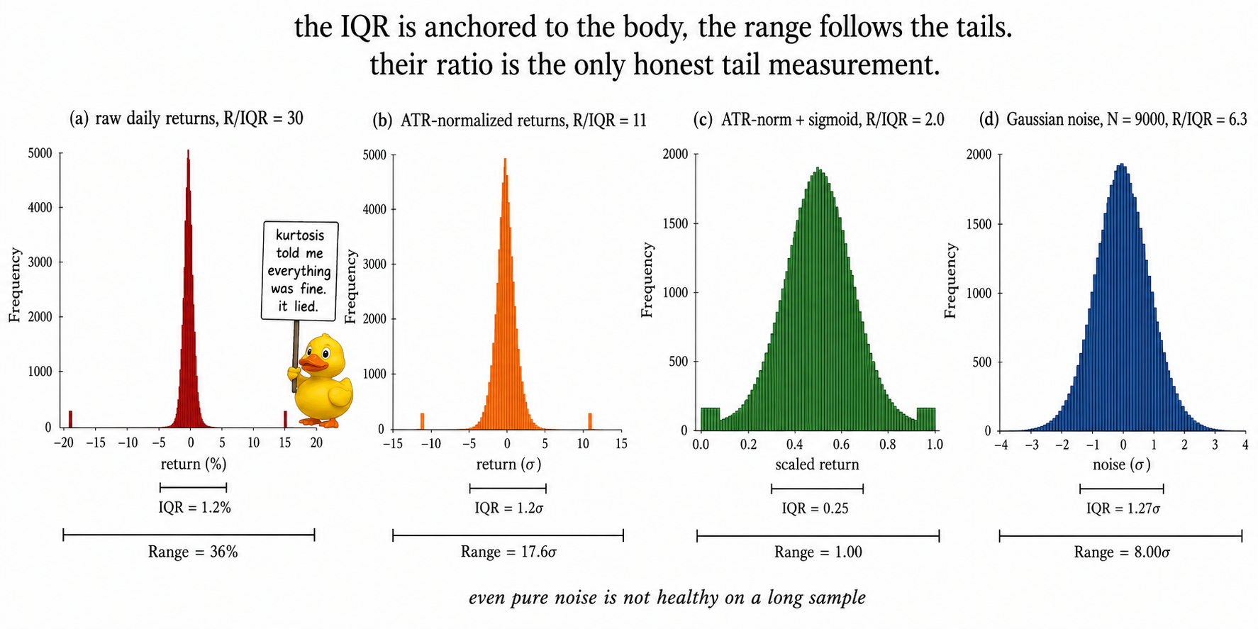
The four panels are the central diagnostic. Three of the four would fail the loss-function-leverage test under least squares. Only one is ready for a model.
What this changes in practice
Three operational shifts.
R/IQR runs first on every candidate feature, before any model touches the data. The computation is two sorted positions for the quartiles, two extremes for the range, and one division. Sub-millisecond on any series. Build it into the indicator-definition phase, not the model-training phase.
The R/IQR of the transformed feature gets logged next to the R/IQR of the raw feature. If the transform did not reduce the ratio, the transform did not address the defect the indicator carried. Replace the transform, do not stack a second one on top.
The Gaussian baseline R/IQR for your sample size sits in a lookup table somewhere in your repo. Comparing your indicator's R/IQR to a fixed cutoff like "5" without considering sample size produces false alarms on short windows and false negatives on long ones. The baseline scales with the square root of log N. Look it up before declaring an indicator clean.
KEY POINTS
- R/IQR is the ratio of the full range of an indicator to its interquartile range. It measures tail extent relative to body width.
- The denominator is anchored to the central 50% of the data and is invariant to any single observation outside the IQR. The numerator follows the extremes. The ratio decouples body measurement from tail measurement.
- Standard deviation and kurtosis both contain the tails inside their own computation. A heavy-tailed indicator inflates both denominator and numerator of any std-based or kurt-based tail metric, so the metric moves slowly when the defect grows. R/IQR does not have this contamination.
- Sample-size dependence: Gaussian R/IQR scales with sqrt(2 log N) divided by 1.349. For N around 9000 the Gaussian baseline is about 6.3. A fixed threshold like "5" is wrong for both short and long series. Use the baseline for your N.
- Operational bands: below 3 is healthy (bounded transforms land here), 3 to 5 is watchlist, 5 to 10 needs a tail-taming transform, above 10 is unusable in raw form.
- Raw price levels score high R/IQR for non-stationarity reasons, not for tail reasons. R/IQR cannot distinguish the two defects. Fix the construction upstream when raw price-based features land in the tail-dominated band.
- Daily SPX returns score R/IQR around 30. ATR-normalization brings it to 11. Sigmoid through a z-scored ATR-norm brings it to 2.0 by construction. The choice between sigmoid and rank depends on whether magnitude information carries signal (covered in "Why Predictive Power Often Lives in the Tails").
- R/IQR misses three defects: bimodal distributions, clumped bodies, and slow drift. Pair it with the relative-entropy quality score and the rolling-moments check from the prior articles.
- The diagnostic belongs to the indicator definition, not the model pipeline. It is computed once at design time and stored with the feature. It does not change when you swap models.
References
- Statistically Sound Indicators for Financial Market Prediction - Timothy Masters (Amazon)
- Cycle Analytics for Traders - John Ehlers (Amazon)
- Using the studentized range to assess kurtosis
- Measuring Skewness and Kurtosis
- Robust measures of skewness and kurtosis for macroeconomic and financial time series
- Looking for skewness in financial time series
- Heavy Tails in High-Frequency Financial Data
- Conditional heavy tails and the stock market returns in Germany
- Higher Realized Moments and Stock Return Predictability
- Kurtosis-based projection pursuit for outlier detection in financial time series