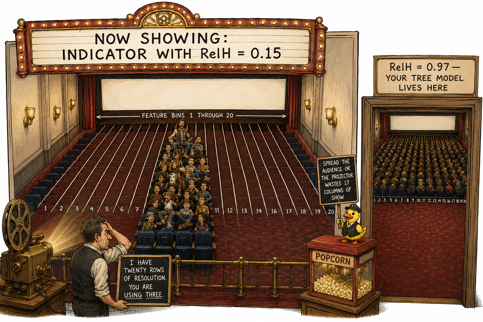
Take an indicator that passes the first three checks from "Garbage Indicators, Garbage Predictions". Its 252-day rolling mean is stable. Its R/IQR sits at 3. ADF rejects the unit root at p < 0.01. Plot the histogram. 96% of the observations sit in 8% of the range. The remaining 4% scatter across the rest of the axis. A tree model with 20 splits available on this feature wastes 18 of them on empty regions and resolves the dense band with two splits. A linear model fits a coefficient calibrated by the empty space and applies it to the dense band where the variation lives.

The first three checks missed the defect. The histogram caught it. "Garbage Indicators, Garbage Predictions" lists distribution shape as the third defect class. The cheapest single-number test for that defect is relative entropy.

What relative entropy means here

Bin the indicator into K bins and let p_k be the empirical probability that an observation falls in bin k. The Shannon entropy of the binned distribution is:

The maximum value of H(X) on K bins is log(K), attained when the distribution is uniform across bins. The relative entropy score is the ratio:

RelH is the fraction of the maximum spread the indicator achieves. RelH = 1 is uniform across bins. RelH = 0 is a delta function in one bin. Healthy indicators sit above 0.8. Raw price-based indicators sit below 0.5.

A terminology note before the rest of the article uses the name. "Relative entropy" in information theory means the Kullback-Leibler divergence between two distributions. The score above is the normalized entropy ratio, not a KL divergence. The two connect:

A low RelH is a large KL from the uniform reference: the indicator's histogram sits far from the maximally-spread shape the model wants. In the rest of this article, "relative entropy" refers to the RelH ratio. "KL" refers to the information-theoretic divergence.

Why model resolution depends on histogram shape

Tree splits and linear coefficients allocate their resolution where the data lives, not where the axis runs. A feature with all of its mass piled in one bin gives the model one usable binary decision on that feature. Variance can be high if a few outliers sit far away from the dense bin, but the model gets no usable resolution in the dense region. Variance is dominated by the outliers. The dense central mass is invisible to it.

Relative entropy counts occupied bins, weighted by occupation density. A clumped distribution has most bins empty and a few bins overloaded. The score drops. The score sees what variance does not.

The operational statement: the model has roughly K possible binary decisions on a feature, where K is the resolution it can extract from that feature. Relative entropy is the fraction of those K decisions that fall in regions with data. A RelH of 0.40 says about 60% of the model's resolution budget on that feature falls in empty space and contributes nothing to the fit.

The binning choice is the only hyperparameter

RelH depends on the binning rule. Three choices and their failure modes.

Equal-width on the full range. Divide the range from min to max into K equal-width bins. One extreme observation stretches the range, so 95% of the bins end up empty and RelH collapses toward zero whether or not the body of the distribution is well-spread. The metric ends up testing for outliers, not for clumping. R/IQR (covered in "Range/IQR: A Simple Test for Indicator Tail Problems") is the right diagnostic for outliers. Relative entropy is the wrong one.

Equal-frequency. Place bin boundaries at empirical quantiles so each bin has the same count. By construction RelH = 1 on any input, including pure white noise and a constant. The metric is degenerate.

Equal-width on a trimmed range. Compute the 1st and 99th percentiles. Discard observations outside that range. Bin the remaining 98% of the data into K equal-width bins on the trimmed window. This is the recommended default and the only choice that does what the score is supposed to do: measure clumping inside the body of the distribution while ignoring the tails. R/IQR catches the tails. RelH catches the body.

K = 20 is the standard bin count for daily-frequency indicators on multi-thousand-observation series. Smaller K hides clumping inside large bins. Larger K starts to register noise in the empirical density estimate. RelH is stable to within ±0.03 across K in the range 15 to 50 on most series. Pick one K and apply it consistently across the candidate indicator set. Sweeping K to find the best-scoring choice is overfitting on the diagnostic.

Worked example: SPX indicators across the transform pipeline

SPX daily, 1990 to 2026. Five candidate features and one noise control. Each scored with K = 20 equal-width bins on the 1st-to-99th-percentile range. Mutual information with the sign of the next-day return is included alongside RelH for contrast.

Three readings from the table.

The raw close scores RelH = 0.41 because price trends across decades pile the post-2010 mass into a few high bins and leave the 1990s bins sparse. The clump sits at the upper end, not in the center, and the histogram is one-sided. "Why Most Indicators Should Be Transformed Before Modeling" already condemned this feature on stationarity grounds. Relative entropy condemns it again on distribution shape. Two independent diagnostics, one verdict.

Each transform step from that article lifts the RelH monotonically: differencing to raw 20-day momentum (0.52), ATR-normalization (0.74), sigmoid through z-scaled ATR-norm (0.92), and rolling rank (0.99 by construction). The progression validates the toolbox. If a transform step does not lift RelH, the transform is not addressing the defect the indicator carried, and the next transform is the wrong call.

The Gaussian noise control scores RelH = 0.96, higher than the ATR-normalized momentum. Its mutual information with the next-day return is 0.0001, indistinguishable from zero. The score says nothing about predictive content. A well-shaped histogram of pure noise scores as well as a well-shaped histogram of signal. The point of the score is not to select indicators that predict. The point is to disqualify indicators whose geometry makes prediction impossible regardless of the underlying signal.

What the score does not tell you

The diagnostic is one-sided. High RelH says the histogram is well-shaped. It carries no claim about whether the indicator predicts anything. The predictive question lives in mutual information against the target, I(X; Y), where Y is whatever you are forecasting. The two scores combine:

Both filters apply. RelH is the cheaper one and runs first: a candidate with RelH = 0.3 gets dropped before any mutual-information computation. A candidate with RelH = 0.9 advances to the MI test.

Two failure modes RelH catches that mutual information misses on small samples. A near-constant indicator with a handful of rare extreme observations can show inflated I(X; Y) if the rare days happen to align with large target moves. RelH on the same indicator sits around 0.05 and disqualifies it: the model cannot resolve where in feature space the rare days came from. A bimodal indicator with the predictive content concentrated in one of the two spikes has moderate I(X; Y) and RelH around 0.30. The model cannot place a decision boundary in the empty middle between the spikes.

Two failure modes RelH misses that MI catches. White noise. Smooth, well-shaped, predictively useless. RelH ≈ 1, MI ≈ 0. And any feature that has been rank-mapped to uniform: RelH = 1 by construction regardless of the underlying signal. Rank transforms pass the geometry test by definition. MI is the only thing that distinguishes a rank-mapped signal from a rank-mapped noise.

The threshold rule

Three bands in practice.

RelH above 0.80. The histogram is well-spread. Pass the indicator on to the mutual-information test and the stationarity tests.

RelH between 0.50 and 0.80. The indicator is salvageable but needs a spreading transform. Sigmoid, fourth-root, or rolling rank from the toolbox in "Why Most Indicators Should Be Transformed Before Modeling". Recompute RelH after the transform. If the score does not lift above 0.80, the underlying construction has structural clumping that no monotonic spread can fix without erasing the magnitude information through a rank transform.

RelH below 0.50. The histogram is concentrated in a small fraction of the range. The cause is almost always non-stationarity in the upstream inputs (raw price, raw volume, or anything else that trends across decades). Either fix the construction at the source or drop the feature. A model trained on a sub-0.5 indicator is allocating most of its capacity to empty space.

These bands are conventions. The 0.5 floor holds up in the SPX, EUR/USD, and CL daily series I have run it on, and in 60-minute and 5-minute resampled versions of the same. The exact cutoff matters less than the principle: rank candidate indicators by RelH, drop the bottom, and spend modeling time on the survivors.

Visualizing the score

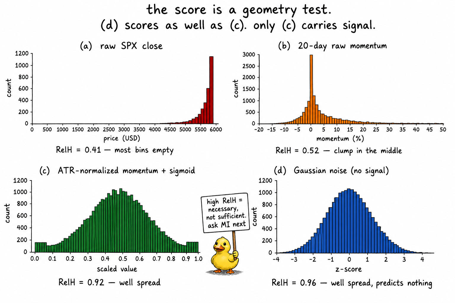
The four panels are the central image. Three of the four pass the score. Two of them carry signal. The score is a precondition, not a verdict.

What this changes in practice

Three operational shifts.

Every candidate indicator gets a RelH number before any model touches it. The computation is one histogram and one entropy sum, milliseconds on a series of any practical length. There is no excuse to skip it. Most retail R&D skips it because the published model libraries do not surface the diagnostic in the default workflow, so it does not exist in the default mental model either.

RelH gets paired with mutual information against the target. The geometry filter (RelH) runs first because it is cheap. The information filter (MI) runs on the survivors. Both are necessary. Either one alone leaks bad indicators into the modeling stage.

The transform pipeline gets validated by RelH at every step. The progression from raw to differenced to ATR-normalized to sigmoid-bounded should produce monotone improvement in RelH. If a transform step does not lift the score, the transform did not address the defect the indicator carried. Replace the transform and retest. The score is the readout that tells you which step did what.

KEY POINTS

• Relative entropy as an indicator quality score is H(X) / log(K), the empirical entropy of the binned indicator divided by the entropy of a uniform distribution on the same bins. It ranges from 0 (delta function) to 1 (uniform across bins).- The score equals 1 minus the normalized KL divergence from a uniform reference. A low score is a large KL from the uniform reference: the histogram sits far from the maximally-spread shape the model needs.
• Variance and RelH measure different things. A clumped distribution with one outlier has high variance and low RelH. Model resolution depends on bin occupancy, not on variance.
• Binning rule choice determines what the score measures. Equal-width on the full range tests for outliers. Equal-frequency is degenerate (always returns 1). Equal-width on the 1st-to-99th-percentile range is the correct choice for clumping.
• K = 20 is the standard bin count for daily indicators on multi-thousand-observation series. The score is stable across K from 15 to 50. Sweeping K to maximize RelH is overfitting on the diagnostic.
• High RelH is necessary, not sufficient. Gaussian noise scores RelH near 1 and carries no signal. Pair RelH with mutual information against the target.
• RelH catches two failure modes MI misses on small samples: rare-extreme indicators where MI is inflated by a handful of aligned days, and bimodal indicators with predictive content in one spike but no resolvable boundary between spikes.
• MI catches two failure modes RelH misses: white noise (high RelH, zero signal) and rank-transformed features (RelH = 1 by construction regardless of content).
• Three operational bands: above 0.80 proceed to MI; 0.50 to 0.80 apply a spreading transform and retest; below 0.50 drop the feature or fix its upstream construction.
• RelH belongs to the feature definition, not to the model pipeline. Compute it once at indicator design time. It does not change when you swap models.