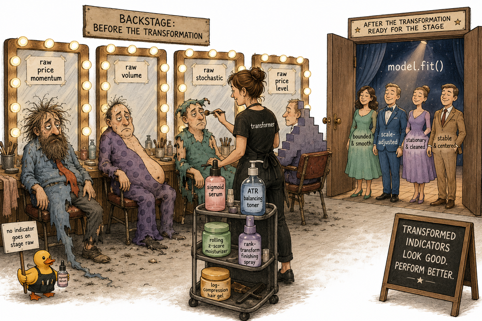
2.3 Why Most Indicators Should Be Transformed Before Modeling
Raw indicators rarely satisfy the geometric assumptions a model needs: stable scale, spread distribution, bounded tails. Six transforms cover most repairs. Each fixes a specific defect, costs a hyperparameter, and risks lookahead if computed non-causally.
You compute a 20-day momentum on AAPL: today's close minus close from 20 bars ago. Across 2010 to 2026, that number ranges from about -$45 to +$60. The standard deviation in 2012 was $1.20. In 2024 it was $11. The mean was $0.30 in 2012 and $1.80 in 2024. You drop this raw indicator into XGBoost. It splits on 4.5, a value that meant "two-sigma move" in 2012 and "below average" in 2024. The split rules carry no time index. The model has learned a 2024 fact and applied it to 2012 data, and a 2012 fact and applied it to 2024.
The indicator was not broken. It was raw. Article 24 cataloged the defects. This article catalogs the repairs.
The four reasons a model needs transformed inputs
A model is a fitting procedure operating on the geometry of the feature space. The geometry needs four things from each feature before the fit becomes reliable.
The values need to live on a stable scale across time. A feature whose typical magnitude in decade A is 1 and whose typical magnitude in decade B is 10 cannot share a decision boundary across both. The model does not know that the underlying market regime changed. It will project the boundary from the larger-scale regime onto the smaller-scale regime and produce nonsense.
The values need to be spread across the range where the model puts its resolution. Tree splits and linear coefficients both default to attending to the spread of the data. If 99% of observations live in 1% of the range, the model carves rules in the empty 99% of the range and treats the dense 1% as uniform.
The tails need to be bounded enough that no single observation dominates the loss. Least-squares loss is quadratic in the residual. A 20σ outlier contributes 400 times what a typical 1σ residual contributes. The fitted coefficients warp around that one point. Tree leaves split at the outliers and treat them as informative regions.
The values need to be comparable across instruments. A 1.5% move in EURUSD and a 1.5% move in BTC do not mean the same thing. A feature that conflates the two cannot be pooled across instruments without scale-mixing the signal.
Most raw indicators fail at least one of these four. Transforming them is what makes the rest of the modeling pipeline honest.
The transform toolbox
Six transforms cover roughly 95% of practical indicator work. Each fixes one or two defects from article 24, and each costs something.
Differencing and returns. Convert a price level into a return: $r_t = P_t/P_{t-1} - 1$, or the log version $\log(P_t/P_{t-1})$. The level was non-stationary by construction (prices trend across decades). The return is approximately stationary for most liquid assets at most horizons. Cost: any information that lived in the level (mean-reversion to a long-term anchor, for example) is gone. Use it as the default first step for anything built on raw price.
Rolling z-score. Subtract a rolling mean and divide by a rolling standard deviation:
The rolling window N is a hyperparameter you now own. The z-score forces local stationarity even when the global series drifts. Cost: you have introduced a window parameter you will be tempted to optimize. Optimization across windows for in-sample fit is overfitting on a transform. Pick N from the time-scale of the indicator (a 20-day momentum gets a 200 to 500-day z-score window, not a 30-day one), not from the backtest.
ATR or volatility normalization. Divide the raw indicator by a rolling measure of dispersion of its underlying price series, usually ATR or rolling return std. A 50-pip move means one thing in low-vol EURUSD and another in high-vol BTC. Dividing by ATR converts both to comparable units. The transformed value is "moves in units of typical local volatility." This is the same idea as a z-score with the location term suppressed, and is often more appropriate for indicators whose natural reference is 0 rather than the rolling mean (price changes, gap sizes, drawdowns).
Log and fourth root. Both compress right-skewed positive variables. Log is harder compression and explodes at zero (use $\log(1+x)$ if the variable can be near zero). Fourth root is gentler and stays defined at zero. Use them for volume, turnover, dollar-traded, and any non-negative variable whose distribution looks like a heavy right tail attached to a dense lump at zero. Cost: both lose information in the tails (a 10x and a 100x outlier become much closer after log). For tail-dependent signals this matters. For loss-function protection, that is the point.
Sigmoid and tanh. Both map the real line to a bounded interval. The sigmoid in standardized form is:
Pass the indicator through a z-score first, then through a sigmoid with scale around 1 to 2. The output lives on [0, 1] with the body of the distribution mapped to the central S-curve and the tails compressed flat at the bounds. This is the most surgical fix for heavy tails because it bounds the loss contribution of any single observation while preserving the rank ordering of the body. Cost: the sigmoid flattens the distinction between a 4σ outlier and a 6σ outlier. If your edge lives in that distinction, the sigmoid destroyed it. Test before committing.
Rank and CDF transforms. Replace each value with its empirical percentile rank in a rolling window. The output is uniform on [0, 1] by construction. This is the most aggressive transform: it discards all distance information and keeps only ordinal information. Two raw values of 0.5 and 5.0 become percentiles 51 and 99 (close in rank space, far in raw space). Use it when the indicator's predictive content is ordinal (extreme values predict reversal, midrange values predict nothing) rather than magnitude-based. Cost: any signal that depended on magnitude is gone, and the rolling window is again a hyperparameter you own.
The defect-to-transform mapping
Article 24's four defects map onto the toolbox.
Defect | Primary fix | Secondary fix |
|---|---|---|
Non-stationary mean | differencing, rolling z-score | ATR normalization |
Non-stationary variance | rolling z-score, ATR normalization | sigmoid with rolling scale |
Heavy tails | sigmoid, tanh, fourth-root | log (for non-negative) |
Clumped distribution | rank, CDF, fourth-root | log (for right-skewed clumps) |
Window artifacts | smoothed lookback (article 39+) | not a transform problem |
The pattern: stationarity defects get rescaled, tail defects get squashed, clumping defects get spread. Each defect has a primary transform that fixes it cleanly and a secondary transform that helps but is less surgical.
What transforms cost
Three costs to track when you reach for the toolbox.
The first is the hyperparameter you just added. A rolling z-score over 200 bars is not the same indicator as one over 500. A sigmoid with scale 1 is not the same as one with scale 2. Each window and each scale is a degree of freedom you can optimize and overfit. Set them from the time-scale of the underlying signal, not from the backtest. Grid-searching rolling-window lengths means you stopped building an indicator and started fitting a hyperparameter to the in-sample data.
The second is the information loss you accepted. Sigmoid destroys the distinction between a 4σ and a 6σ event. Log destroys the distinction between a 10x and a 100x outlier. Rank destroys all magnitude information. If your edge depended on the thing the transform threw away, you have made the indicator worse, not better. Check this with relative entropy or mutual information against the target before and after the transform (article 26 walks through the score). The transform should leave the target relationship intact while reshaping the distribution.
The third is lookahead. A z-score that uses the full-sample mean and std is computed with knowledge of the future. So is a CDF transform that uses the full-sample empirical distribution. Every transform that touches a distribution statistic must be computed in a rolling, causal way. The naive sklearn StandardScaler fit on the full training set and applied to the test set leaks future information into the test set in time-series problems. The fix is rolling-window versions of every transform, with the window strictly preceding the prediction bar.
Worked example: SPX 20-day momentum across four transforms
SPX, 1990 to 2026. Target is the sign of the next-day return. ADF is the Augmented Dickey-Fuller test for a unit root; rejecting at p < 0.05 means we treat the series as stationary.
The model class never changed. The spread across rows (2), (3), (4) is the transform-choice question: ATR-norm alone captures most of the gain; sigmoid edges higher because it preserves the gradient in the body while bounding the tails; rank does about the same with a different information trade (all magnitude information discarded, only ordering kept). The right transform depends on whether the body or the tails carry the edge, which is something you measure (article 26's relative entropy score, article 28's tail diagnostics), not guess.
Visualizing the four transforms
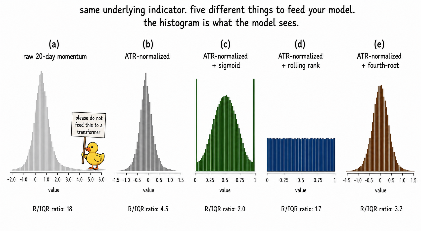
The five histograms are the central image. The indicator carried roughly the same information across all five. The change is whether the model could use it.
What this changes in practice
Three operational shifts.
Every indicator gets diagnosed (article 24's four checks) and transformed before any model training. Default order: stationarize first, then tame tails, then check distribution shape. Skipping the diagnosis means you do not know which transform to apply, so you guess, and the guess is usually wrong.
The transform is part of the indicator, not part of the model pipeline. A 20-day ATR-normalized momentum is a different indicator from a 20-day raw momentum. Treat them as separate features in your research log. The transform's hyperparameters (rolling-window length, sigmoid scale) belong to the feature definition, not to free knobs you sweep at backtest time.
Causal computation is non-negotiable. Every rolling statistic, every rolling rank, every rolling z-score uses only past data. Lookahead bias from a non-causal transform is the single most common reason a research backtest looks great and the live equity curve does not. Fix it at the transform layer, before any model sees the data.
KEY POINTS
- A model needs four things from each feature: stable scale, spread distribution, bounded tails, and cross-instrument comparability. Most raw indicators fail at least one of the four.
- Six transforms cover most practical work: differencing, rolling z-score, ATR normalization, log and fourth-root, sigmoid and tanh, and rank/CDF.
- The defect-to-transform mapping is mechanical. Non-stationarity gets rescaled. Heavy tails get squashed. Clumping gets spread. Each defect has a primary fix and a secondary fix.
- Every transform has a cost: a hyperparameter to set, information loss in the part of the distribution the transform compresses, and a risk of lookahead if the statistics are computed non-causally.
- Sigmoid preserves the gradient in the body while bounding the tails. Use it when the edge lives in the central distribution and the tails are noise.
- Rank discards all magnitude information and keeps only ordinal content. Use it when the edge is ordinal (extremes predict reversal) rather than magnitude-based.
- The hyperparameters of a transform (window length, sigmoid scale) belong to the feature definition. Optimizing them on the backtest is overfitting on the transform.
- Every rolling statistic must be computed causally. Full-sample StandardScaler on a time series leaks future information and inflates backtest performance.
- Use mutual information or relative entropy (article 26) against the target to check that the transform reshaped the distribution without destroying the signal.
- The improvement from a transform is usually larger than the improvement from a model upgrade. The model class is the constant. The indicator transform is the variable.
References
- Statistically Sound Indicators for Financial Market Prediction - Timothy Masters (Amazon)
- Cycle Analytics for Traders - John Ehlers (Amazon)
- Financial Signal Processing and Machine Learning
- Technical Indicator Networks (TINs): An Interpretable Neural Architecture for Financial Technical Analysis
- Reasoning on Time-Series for Financial Technical Analysis
- Hierarchical Endogenous Market-State Representation for Financial Time Series
- Financial Time-Series Prediction Using Deep Learning
- Recurrence Interval Analysis of Financial Time Series
- Digital Signal Processing System Analysis and Design (excerpt with financial-indicator examples)
- Financial Signal Processing and Machine Learning (publisher page)