Pick a popular volume indicator and plot it across twenty years of SPY. Mean in 2003: roughly 80 million shares. Mean in 2024: roughly 70 million shares, but with two regime shifts and a five-fold spike in 2020. The standard deviation tripled, halved, and tripled again. You train a model on the 2003–2018 distribution. You deploy on the 2024 distribution. The "indicator" you fed the model in training did not exist in production. The model is now mapping new inputs through the wrong function. It will lose money in a structurally consistent way until you turn it off.

This is what garbage looks like. The indicator did not have a noisy correlation. It had a defect. Articles in this pillar split into two halves: how to diagnose the defects, and how to repair them. This article is the catalog. The repairs come in articles 25 through 38.

What "garbage" means operationally

A garbage indicator is one of four things, sometimes more than one at once.

1. The distribution drifts over time. The mean in decade A is different from the mean in decade B. The variance shifts. A model trained on A predicts using statistics that no longer apply in B.
2. The distribution has outliers heavy enough to dominate the model's loss function. The model spends its parameter budget fitting three days from 1987 and 2008 instead of the central 99% of observations.
3. The distribution has values clumped into narrow bands separated by wide empty regions. The model carves rules in the empty regions where there is no data, and ignores the dense clumps where the predictive content sits.
4. The indicator construction injects artifacts. The lookback window flips, sign-inverts, or wildly rescales the indicator at points unrelated to anything the market did.

None of these defects can be fixed by switching from logistic regression to a transformer. The model class does not see the defect. The model sees what you fed it and treats it as the truth. The defect propagates into the forecast.

Failure mode 1: non-stationarity

You compute an indicator on SPX from 1990 to 2026. You plot its rolling 252-day mean. If that mean wanders from 12 in 2000 to 480 in 2024, the indicator's distribution in 2000 has nothing to do with its distribution in 2024. The same numerical value carries opposite information in the two regimes. A 50 in 2000 was an extreme. A 50 in 2024 is below the floor. Any model trained across both regimes is averaging contradictions.

Stationarity is the requirement that the statistical properties of an indicator stay roughly constant across time. It is the floor on indicator usability, not a polish step. You cannot train on past samples and deploy on future ones if the past samples are not drawn from the same distribution as the future ones. The bridge between training and live trading is the assumption of stationarity. Break the assumption and you break the bridge.

Three diagnostics catch most non-stationarity in practice.

Plot a rolling mean over a window long enough to average out short-term noise (200 to 500 bars). If the rolling mean wanders monotonically or has visible regime breaks, the indicator is non-stationary in the first moment.

Plot a rolling standard deviation or IQR over the same window. If the spread expands or contracts across decades, the indicator is non-stationary in the second moment. This is the more common defect and the more dangerous one because models tend to under-react to it.

Run an Augmented Dickey-Fuller test on the indicator series. If the test fails to reject the null of a unit root at p < 0.05, treat the indicator as suspect and look for a construction that produces a stationary version.

The repair is upstream. Indicators built directly on raw price levels, raw volume, or anything else that trends across decades inherit the non-stationarity of their inputs. Indicators built on returns, ratios, percentile ranks, ATR-normalized differences, and rolling z-scores tend to be stationary by construction. Article 32 walks through the conversions.

Failure mode 2: heavy tails and outliers

Take SPX one-day returns from 1928 to 2026. The max is around +16% (1933). The min is around -20% (1987). The interquartile range across the full sample is around 0.012. The range over IQR ratio:

R/IQR of 30 means the extreme values stretch the range to thirty times the width of the central half of the data. A reasonable indicator sits at R/IQR between 2 and 3. Anything above 5 is dominated by tails. At 30, the indicator is not a feature, it is a list of crashes with some noise around them.

Heavy tails corrupt models in three measurable ways. The least-squares loss is quadratic in the residual, so a single outlier of magnitude 20σ contributes 400 times what a typical 1σ residual contributes. The fitted coefficients warp to absorb that one observation. Tree-based models split the feature space at the outliers, producing leaf nodes with one or two samples that get treated as informative regions. Standardization (subtracting mean, dividing by standard deviation) is also corrupted because the standard deviation is pulled up by the outliers, so the rescaled values for the central 99% of observations get compressed into a narrow band where no model can resolve them.

The diagnostic is the R/IQR ratio itself. Compute it on every candidate indicator before you compute anything else. If R/IQR is above 5, the indicator needs a tail-taming transform: a fourth-root for mild compression, log for moderate compression, or a sigmoid for hard bounds. Articles 33 and 36 walk through the choices and their distortions.

Failure mode 3: clumped distributions

You build an indicator whose histogram has one tall spike near zero and a long thin tail to the right. Most days the indicator reads 0.01 to 0.05. A few days a year it reads 2 to 5. The model sees a feature that is approximately constant 99% of the time. It carves its decision boundary in the tail where it has fifteen training samples. It treats the dense central mass as a flat region with no information.

The predictive content of the indicator may actually live in the clump, not in the tail. Models default to attending to the spread because the spread is where the variance is. Variance is not the same as information. A clumped distribution can hide rich structure inside the clump that the model never resolves because the resolution of its decision rules is set by the global scale of the feature.

The diagnostic is visual and entropic. Plot the histogram with enough bins to see the shape (50 to 200 bins, depending on sample size). Look for one tall narrow spike, two spikes separated by emptiness, or a long thin tail attached to a dense ball. Then compute the differential entropy of the distribution after binning, normalized by the entropy of a uniform distribution with the same range. A value below 0.5 indicates the data is concentrating in narrow regions. Article 26 turns this into a quality score.

The repair is a monotonic transform that spreads the clump out: rank transforms, fourth-root for mild spread, or a CDF transform that maps the empirical distribution to uniform. The transformed indicator carries the same information by the data-processing inequality, but the model can now resolve it.

Failure mode 4: construction artifacts

The raw stochastic oscillator computes (close - low) / (high - low) over a lookback window. As the window rolls forward by one bar, the oldest bar drops out and the newest one enters. If the dropping bar was the high or low of the window, the denominator changes discontinuously. The indicator value jumps even if the close did not move. Across thousands of bars, the indicator carries as much window-artifact noise as it does market signal.

Most indicators built on lookback ranges have a version of this defect. Bollinger bands have it on the standard deviation. Donchian channels have it on the high and low. Any rule of the form "compare today to the extreme of the last N bars" inherits the discontinuity at the edges of the window.

The diagnostic is to compute the indicator twice: once with lookback N, once with lookback N+1. If the two series diverge by more than the underlying price moved, the indicator is reading the window, not the market. Article 23's smoothing discussion and articles 39 onward on filter design give the alternative: indicators built on smoothed weighted averages of the lookback range, not on the raw extreme values, are less brittle at the window edges.

Why the defects compound

A model trained on a non-stationary, heavy-tailed, clumped indicator with window artifacts is not failing on four small problems. It is failing on a single composite problem where each defect masks the others. The non-stationarity makes the heavy tails look like signal because the tails align with regime breaks. The clumping hides the non-stationarity because the rolling mean stays inside the same dense band even as the underlying distribution shifts. The window artifacts get absorbed into the model's noise floor and inflate the standard error of every estimated coefficient.

The result is a strategy whose in-sample Sharpe looks fine, whose out-of-sample Sharpe is half of in-sample, and whose live Sharpe is half of out-of-sample. Each of the three drops is a defect compounding through the deployment chain.

Visualizing what bad distributions look like

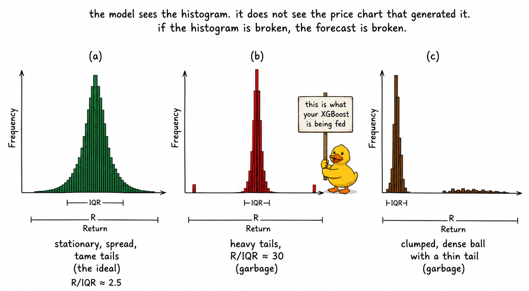
The three histograms are the central diagnostic. Look at the shape before you look at the backtest.

What this changes in practice

Compute four numbers on every candidate indicator before you train a model.

The rolling mean and rolling standard deviation across the full sample, plotted as two time series. Eyeball them for drift and regime breaks. Run an ADF test if the visual is ambiguous.

The R/IQR ratio across the full sample. If it is above 5, you have a tail problem. If it is above 10, the indicator is unusable in its raw form.

The histogram with 50 to 200 bins. Look for clumping, gaps, and asymmetries that no monotonic transform will fix without losing information.

A consistency check by perturbing the lookback by ±1 bar. If the indicator jumps, you have a window artifact.

These four checks take five minutes of code each and rule out 80% of bad indicators before any model touches them. Most retail R&D skips them because the tools point in the other direction (model libraries are convenient, indicator diagnostics are not packaged). Most performance is left on the table at this step.

KEY POINTS

• A garbage indicator has one of four structural defects: non-stationary distribution, heavy tails, clumped values, or construction artifacts from lookback windows.
• Switching models does not fix any of these defects. The model treats the input as the truth. The defect propagates into the forecast unchanged.
• Stationarity is the precondition for any prediction. If the indicator's mean or variance drifts across decades, the model trained on one decade is predicting the wrong thing in the next.
• R/IQR is the cheapest tail diagnostic. Below 3 is healthy, above 5 needs a tail-taming transform, above 10 is unusable in raw form.
• Clumped distributions hide predictive content inside dense regions where models default to ignoring it. Monotonic spreading transforms (rank, root, CDF) recover the information.
• Lookback-based indicators (stochastic, Bollinger, Donchian) carry window artifacts whose magnitude can exceed the market signal. Perturb the lookback by one bar to detect this.
• Defects compound. Non-stationarity, heavy tails, and clumping together produce a strategy where each defect masks the others, and the live Sharpe is a fraction of the in-sample one.
• Four diagnostic checks (rolling moments, R/IQR, histogram shape, lookback perturbation) take twenty minutes and rule out most bad indicators before a model is involved.
• The repair lives upstream of the model. Stationary construction, tail transforms, spreading transforms, and smoothed lookbacks. Articles 25 through 38 work through each.