Most trading strategies fail in live markets because the development process skipped steps. The skip is not deliberate. It is the default. The default process is to find a pattern, run a backtest, see a number, and ship. The result is a strategy that performs well in the sample it was built on and badly in the sample it will be deployed against.

The scientific method is the alternative. It is not a philosophy. It is an engineering protocol with explicit stages, pass/fail gates, and decision criteria. The protocol is demanding by design. Most candidate strategies die in the middle. The few that survive all stages have earned the only kind of confidence that survives contact with live markets: confidence based on rigorous pre-committed falsification attempts that the strategy passed.

This article closes the Scientific Trader pillar by integrating the tools from the previous articles into a single end-to-end workflow. Each stage references the article that handled the underlying machinery.

The eleven stages

The protocol has eleven stages. Each stage has a pass criterion and a stop criterion. A strategy that fails the stop criterion at any stage is discarded or reformulated. A strategy that passes all eleven stages is ready for live deployment.

Stage 1. Observation

A candidate phenomenon is identified. The source can be real-world experience (a market behavior the trader has noticed), published research, a structural feature of the market (settlement effects, expiration cycles, central bank announcements), or anomaly detection on data.

Stop criterion: the phenomenon cannot be described in precise words. If the candidate is "stocks tend to go up after a news event but only when the mood is right," the observation has not yet been articulated.

Stage 2. Hypothesis formulation

The observation is transformed into a falsifiable hypothesis (the seven-step transformation in article 19). The hypothesis names a specific variable, a specific condition, a specific horizon, and a specific direction. It can be coded into a deterministic function that two independent researchers running on the same data compute identically.

Stop criterion: the hypothesis cannot be coded. It is still subjective, still time-unbounded, or still result-dependent. Return to Stage 1 or discard.

Stage 3. Null hypothesis specification

The null hypothesis is defined (article 16). For a trading rule, the canonical null is "the rule has no predictive power; its expected return on detrended data is zero or negative." The null model that will be simulated must be specified: bootstrap, block bootstrap, signal permutation, or factor regression.

Stop criterion: the null cannot be made realistic. The trader cannot construct a generator of "this rule under no edge" that respects the volatility clustering, autocorrelation, and fat tails of the underlying market data.

Stage 4. Test statistic and decision rule

A test statistic is chosen (mean return per signal, Sharpe ratio, hit rate, or information ratio against the primary benchmark). An α threshold is committed to. The standard is 0.05; for live-capital decisions, stricter values (0.01 or 0.005) are appropriate (article 16).

Stop criterion: either choice is post-committed. If the test statistic or threshold is left flexible until after the result is seen, the test has no scientific value.

Stage 5. Backtest construction

The backtest is built with the constraints that distinguish an experiment from a screenshot (article 12). Point-in-time data, no lookahead, realistic transaction costs and slippage, detrending of market returns, and explicit benchmarks (article 17).

Stop criterion: any of these constraints is violated. A backtest with lookahead, no costs, or no benchmark is decoration, not data.

Stage 6. Statistical inference

The test statistic is computed on the actual backtest. The same statistic is computed on thousands of simulations from the null model. The p-value is the fraction of null simulations that produced a statistic at least as extreme as the observed one. The 95% confidence interval on the effect size is computed from the bootstrap (article 13).

Pass criterion: p < α AND the lower bound of the CI on the effect size is meaningfully positive (not just barely above zero).

Stop criterion: p > α OR the CI contains zero. The strategy has not falsified the null. Discard.

Stage 7. Bias decomposition

The six diagnostic tests from article 18 are run: detrended re-run, signal permutation, bias-matched random rule, regime split, factor regression, and instrument swap. Each test isolates a different form of hidden bias.

Pass criterion: residual alpha remains after every exposure is stripped out. The strategy's edge is not driven by sector tilt, factor exposure, regime selection, or any other implicit bias.

Stop criterion: any diagnostic reveals that the apparent edge is actually exposure. Discard.

Stage 8. Robustness validation

Three robustness checks (article 7).

Cross-instrument: the rule works on related markets with reasonable parameter values, not only the original instrument with hand-picked parameters.

Cross-period: the rule works on different sub-windows of history, including ones that contain different volatility and trend regimes.

Cross-parameter: small perturbations of the parameters do not destroy the edge. The performance surface in parameter space is smooth, not spiky.

Pass criterion: the rule produces positive results across instruments, periods, and parameter perturbations. The edge is loose pants, not skin-tight.

Stop criterion: the rule's performance is sharply localized to specific parameter values, specific instruments, or specific time windows. Discard.

Stage 9. Walk-forward and paper trading

The rule is implemented as production code. The code is walk-forward-tested with rolling re-fits (parameters re-estimated periodically using only data available before the trade date). The code runs in a paper-trading mode on live data for a calibration period (typically several weeks to several months depending on signal frequency).

Pass criterion: walk-forward performance is consistent with the backtest distribution. Paper-trading execution matches the backtest in fill rates, slippage, and timing.

Stop criterion: execution behavior differs from backtest assumptions, signals fire at different times than expected, or walk-forward performance is well below backtest performance.

Stage 10. Live deployment with monitoring

Capital is allocated. The size respects the wider true uncertainty captured in articles 13 and 14: the backtest's confidence interval is the lower bound on uncertainty, and the live confidence interval is wider because of regime drift and non-stationarity.

Every signal, every trade, every fill, every P&L attribution is logged. Live performance is compared to the backtest's confidence interval continuously. Kill criteria are defined in advance.

Pass criterion: live performance falls within the backtest's 95% CI over the monitoring window.

Stop criterion: live performance falls outside the CI for a sustained period (typically defined as a number of consecutive months or a cumulative drawdown threshold). The strategy is paused.

Stage 11. Iteration and falsification in production

The hypothesis remains provisionally accepted only as long as live data continues to support it. Markets are non-stationary (article 14). An edge that was real in the backtest period may dissipate, reverse, or change shape in live trading. The protocol must be re-run periodically as more data accumulates.

When live performance falls outside the expected distribution for a sustained period, the hypothesis is rejected. The honest response is to discard or reformulate the strategy. The dishonest response is to "tweak parameters until live works again," which is in-sample fitting on the live data and produces the same overfitting problem the protocol was designed to avoid.

The integrated decision rule

A strategy ships only if every stage passes. Formally:

The conjunction is the entire pipeline. A single stage failure stops the strategy.

If the tests are approximately independent and the null hypothesis is true (the strategy has no edge), the probability of false-shipping a worthless strategy through the full pipeline is roughly the product of the individual stage failure rates:

With even a modest N at α = 0.05 per stage, the joint false-positive rate is tiny. The tests are not fully independent in practice, so the real rate is higher, but the principle holds: stacking pre-committed tests produces multi-layer protection against false positives that no single test can deliver.

The cost of the protocol is that many genuine edges are also rejected. This is the Type II error from article 16. The trade-off is accepted because Type I errors (worthless strategies in live trading) consume capital, attention, and confidence, while Type II errors (real edges that were missed) cost only opportunity.

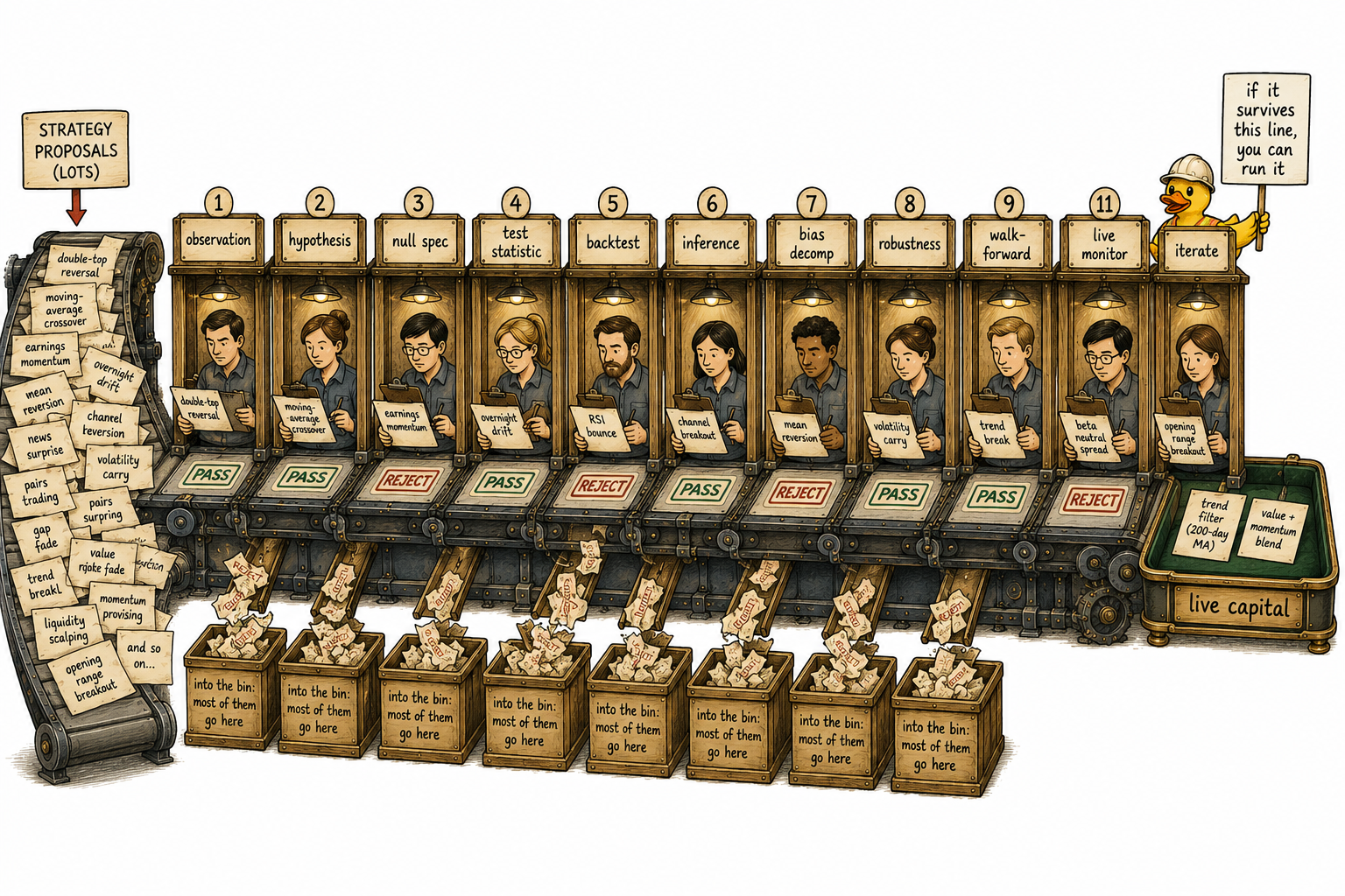
Visualizing the pipeline

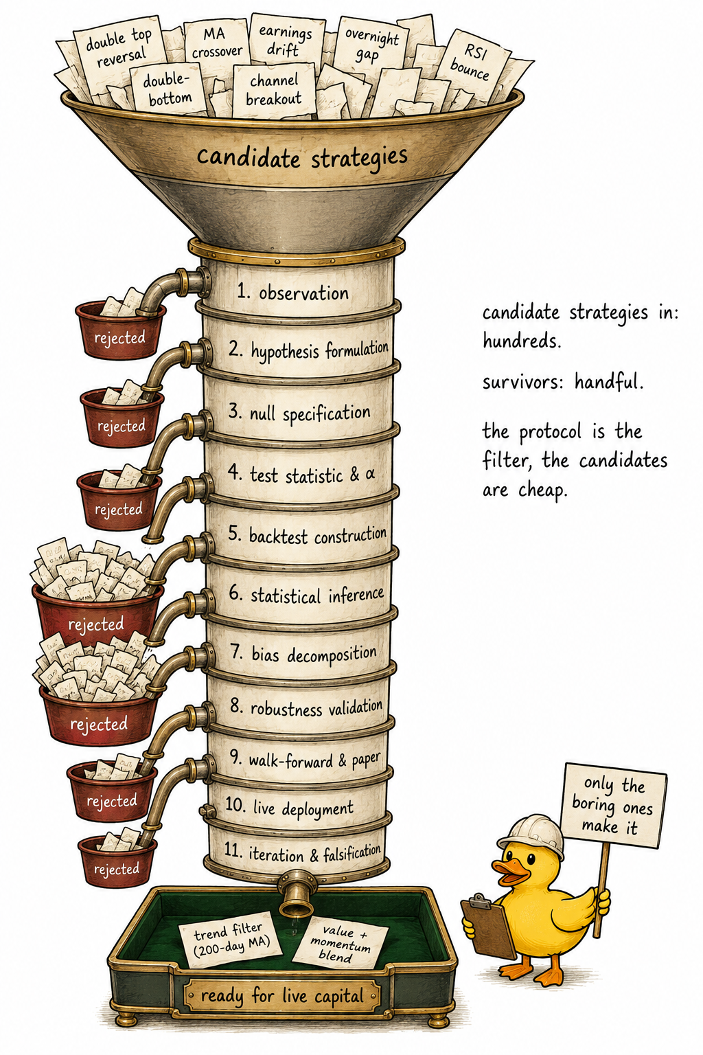
The picture is the entire article. Hundreds of candidate strategies enter the funnel. A handful exits to live capital. Each stage is a gate that filters the candidates that fail its criterion.

Why most strategies fail this protocol

The protocol is demanding by design. The empirical observation across decades is consistent: most apparent trading edges are noise, bias, selection effects, or factor exposures that look like edge. Each stage is calibrated to detect one or more of these failure modes.

Stage 6 (statistical inference) eliminates strategies whose backtest performance is consistent with chance. Stage 7 (bias decomposition) eliminates strategies whose returns are explained by hidden exposures. Stage 8 (robustness validation) eliminates strategies that are narrowly fit to one instrument, one period, or one parameter set. Stage 9 (walk-forward) eliminates strategies that work in idealized backtests but not in realistic execution. Stage 10 (monitoring) eliminates strategies whose live behavior diverges from the backtest, even if they passed every earlier stage.

The strategies that survive all eleven stages are rare. They are also unglamorous. They tend to have few parameters (article 21), modest backtested Sharpe ratios, and broad generalization across instruments and periods. They look unimpressive next to the unfiltered candidates with backtested Sharpe ratios of 3.0 that died at Stage 7. They are the only strategies that pay in live trading.

The role of iteration

Science is not a single test. It is a continuous process of falsification and refinement. Even strategies that pass the full protocol will eventually be falsified by changing markets. An edge that worked in the backtest sample because of a specific market structure (low rates, tight spreads, retail dominance, market-maker behavior, regulatory regime) may stop working when that structure changes.

The protocol must be re-run periodically on live data. New observations are appended to the historical record. The null hypothesis test is recomputed with the larger sample. The bias decomposition is rerun in case new exposures have emerged. The robustness checks are repeated against the new regimes.

A strategy that fails the re-run is paused. The hypothesis has been falsified by the new data. The honest response is to acknowledge the falsification and either reformulate or retire the strategy. The dishonest response is to retroactively change the protocol to keep the strategy alive. This is the same overfitting move the protocol was designed to prevent, applied to live data instead of backtest data, and it produces the same result.

A living strategy is one that continuously survives re-falsification. Most strategies do not last for decades. A few do. The ones that do are the ones whose underlying mechanism is general enough that it transcends specific market regimes (article 7's loose-pants principle), and they survive precisely because their generality makes them robust to regime change.

What this changes for the practitioner

Three operational shifts.

Codify the protocol as a checklist in the development environment. Every candidate strategy passes through every gate, in order, with explicit pass/fail outcomes logged for each stage. No shortcuts. No skipping. No moving the gate after a strategy stumbles. The checklist is the contract between the trader and the trader's future self, who will be tempted to ship a beautiful backtest without doing the work.

Accept that the survival rate will be low. For every published anomaly that becomes a real strategy, dozens die in the middle of the pipeline. The development process is not "find a strategy." It is "filter candidates until one survives." The candidates are cheap. The filter is the value.

Re-run the protocol on live strategies periodically. The strategies that earn capital next year are the ones that pass the protocol next year, regardless of how they performed last year. A strategy that returned 18% per year for a decade and falls outside its confidence interval in the eleventh year is a strategy that has been falsified by the new data. The honest response is to pause and re-evaluate, not to assume the eleventh year is noise.

KEY POINTS

• The scientific method for trading is an eleven-stage protocol with explicit pass/fail criteria at each stage. The protocol is demanding by design and filters most candidate strategies.
• The stages are: observation, hypothesis formulation, null hypothesis specification, test statistic and decision rule, backtest construction, statistical inference, bias decomposition, robustness validation, walk-forward and paper trading, live deployment with monitoring, and iteration and falsification in production.
• Each stage is supported by machinery developed earlier in this pillar. Stage 2 uses article 19, Stage 3 uses article 16, Stage 5 uses articles 12 and 17, Stage 6 uses article 13, Stage 7 uses article 18, Stage 8 uses article 7, Stages 10 and 11 use articles 13 and 14.
• A strategy ships only if every stage passes. The joint false-positive rate of stacked pre-committed tests is far lower than any single test, providing multi-layer protection against shipping worthless strategies.
• The protocol accepts a higher Type II error rate (real edges missed) in exchange for a much lower Type I error rate (worthless strategies shipped). The asymmetry favors strictness because Type I errors cost capital and Type II errors cost only opportunity.
• The strategies that survive all eleven stages are rare and unglamorous: few parameters, modest Sharpe ratios, broad generalization. They are the only strategies worth running.
• The protocol is not a one-time gate. Markets are non-stationary, so strategies must be re-evaluated periodically. The honest response to live failure is to discard or reformulate, not to tweak parameters until live performance returns.
• A living strategy is one that continuously survives re-falsification. The strategies that last for decades have underlying mechanisms general enough that they transcend specific market regimes.
• Operational fix: codify the protocol as a development checklist, run every candidate through every gate, accept low survival rates, and re-run the protocol on live strategies as new data accumulates.