The prior article in this series ("The Case Against Raw Price Indicators") rejected raw close, raw moving averages, and raw band envelopes at the feature-design stage. The argument was structural: non-stationary mean, non-stationary variance, no cross-instrument comparability, and a guaranteed extrapolation failure once live prices leave the training support.

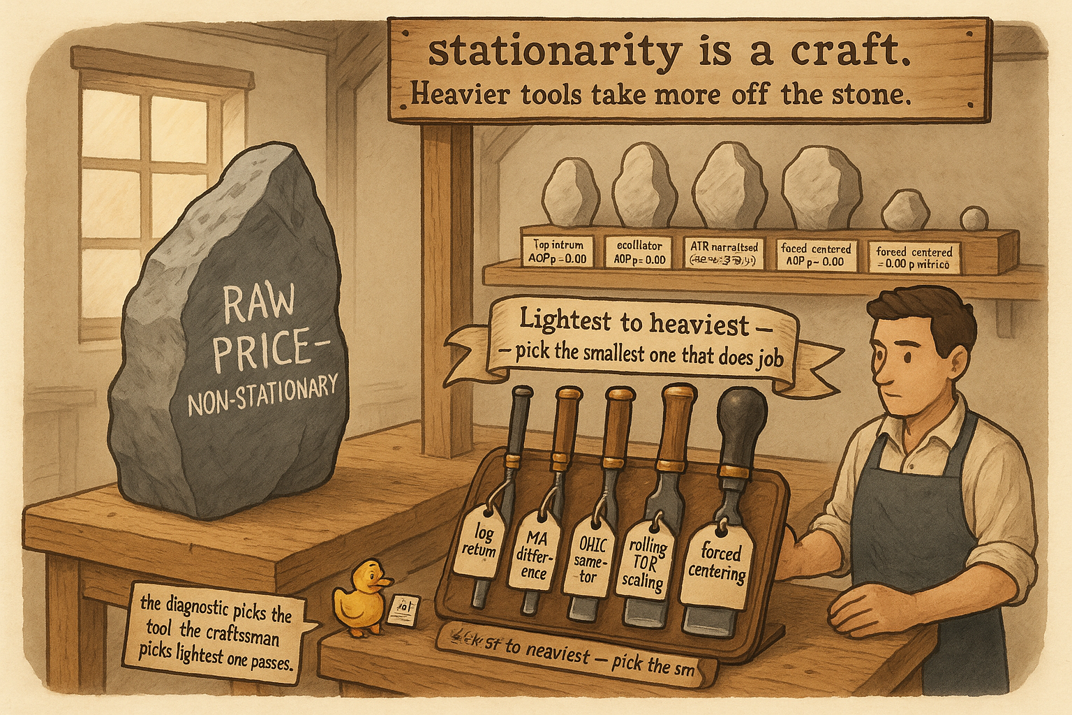
That article ended at the diagnostic. This one is the recipe. Six transforms, in increasing order of how aggressively they kill non-stationarity, with the explicit trade that each transform discards information about the raw price level along with the non-stationarity it removes. Pick the lightest transform that passes the diagnostics, not the heaviest one.

The ATR-normalization case (transform 5 below) is covered in depth in the next article in this series ("Why ATR Normalization Is More Than a Volatility Trick"). The summary appears here; the structural argument lives there.

The stationarity-information tradeoff

Every transform that removes non-stationarity from a price series discards some part of the raw level information that the original series carried. The tradeoff is structural and unavoidable. The ranking by aggressiveness, from lightest to heaviest:

$$ \begin{array}{l|c|c|l} \text{Transform} & \text{Removes mean drift} & \text{Removes variance drift} & \text{Information discarded} \\ \hline \text{Log return } r_t = \ln(P_t / P_{t-1}) & \text{yes} & \text{partial} & \text{absolute level} \\ \text{Oscillator } X_t - X_{t-k} & \text{yes (if } k \text{ moderate)} & \text{partial} & \text{slow-trend level} \\ \text{Same-bar OHLC diff} & \text{yes (by construction)} & \text{no} & \text{intra-bar absolute scale} \\ \text{Direct variance scaling: } X_t / \text{IQR}_t & \text{no} & \text{yes} & \text{absolute magnitude} \\ \text{ATR-normalized diff: } (X_t - X_{t-k}) / \text{ATR}_t & \text{yes} & \text{yes} & \text{level and absolute magnitude} \\ \text{Forced centering: } X_t - \text{median}_{t,W} & \text{yes (aggressive)} & \text{no} & \text{the full level, including useful drift} \\ \end{array} $$

The right transform for a given indicator is the lightest one that produces a series passing the three diagnostics from the prior article: ADF p ≤ 0.05, train-test feature-range coverage ≥ 95%, and rolling 252-bar mean drift below one in-sample standard deviation.

Transform 1: Log returns and first differencing

The default starting point. r_t = ln(P_t / P_{t-1}) converts a non-stationary price series into a stationary return series for all practical equity, FX, and most futures markets.

Two structural properties matter.

The log return is additive across time: ln(P_t / P_{t-k}) = sum of the k single-step log returns. The k-step return and the 1-step return live in the same units and can be modeled jointly. The simple percentage return P_t / P_{t-1} − 1 does not have this additivity and breaks for any multi-step compounded analysis.

Log returns absorb the proportional structure of price moves. A $5 move on a $50 stock and a $50 move on a $500 stock produce the same log return. A pooled cross-sectional model on log returns has comparable features across instruments without further normalization. The article "The Case Against Raw Price Indicators" covered the cross-instrument incomparability of raw prices; log returns remove it at the construction step.

The residual non-stationarity in log returns is variance, not mean. Equity index log returns have stationary mean (close to zero) but non-stationary variance (volatility clustering, regime shifts). The ADF test on SPX daily log returns passes by a wide margin. The variance ratio test detects the variance non-stationarity, which is the cue to apply a variance-scaling transform on top.

Transform 2: Oscillators built from two prices

The construction subtracts two quantities that share the same drift, so the difference is stationary in mean by construction.

$$ O_t \;=\; \text{MA}_n(P_t) \;-\; \text{MA}_m(P_t), \qquad n < m $$

The fast moving average MA_n tracks the recent price level. The slow moving average MA_m tracks the slower-moving level. The drift in P_t enters both quantities at almost the same rate, so the subtraction nets it out. If the mean drifts up or down, the act of subtraction cancels out most of the mean drift.

Two construction details determine whether the oscillator is stationary.

The lag separation should be moderate. n = 10 and m = 50 produces a small enough gap that the two MAs share most of their drift. n = 2 and m = 200 produces a gap large enough that the long MA is structurally lagging the short MA by 100 bars on average, and the difference accumulates the trend over that span. The "large difference of lags" case fails the ADF test on trending instruments.

The same-indicator-with-lag variant works similarly. RSI(14)t − RSI(14){t−14} is stationary because RSI is bounded and the subtraction removes any slow drift in the rolling RSI mean. This construction discards the absolute RSI level (whether the market is in an overbought regime overall) but keeps the change in regime, which is usually the predictive part.

The residual non-stationarity is variance. The oscillator's variance scales with the variance of the underlying price moves, so volatility regimes leak through. Apply transform 4 or 5 on top.

Transform 3: Same-bar OHLC differences

The construction takes two prices recorded on the same bar (same minute, same day), so the drift between them is structurally zero.

$$ \text{Range}_t = H_t - L_t, \quad \text{UpperShadow}_t = H_t - \max(O_t, C_t), \quad \text{Body}_t = |C_t - O_t| $$

The same-bar drift between H and L is zero by construction. There is no calendar offset between the two quantities. The difference has no mean drift regardless of how the underlying price level evolves.

The variance is still non-stationary because the absolute range scales with the price level. A $5 daily range on a $50 stock is large; a $5 daily range on a $500 stock is small. The fix is to normalize by either the bar's own midpoint (Range_t / ((H_t + L_t) / 2)) or by an external scale (ATR over a long window).

The normalized same-bar OHLC differences are some of the most stationary primitives available: Body / Range, UpperShadow / Range, Range / ATR. All three are bounded, drift-free, and comparable across instruments. The Stochastic K indicator is a same-bar OHLC primitive at heart: (Close − Low_n) / (High_n − Low_n) over a lookback n. The reason Stochastic K is stationary is the same reason any same-bar OHLC ratio is stationary.

Transform 4: Direct variance scaling

The construction divides the indicator by a rolling measure of its own variation. The mean stays where it was; the variance is forced toward unity.

$$ \tilde{X}_t \;=\; \frac{X_t}{\sqrt{\text{IQR}_{W}(X)_t}} \quad \text{or} \quad \frac{X_t}{\text{std}_W(X)_t} $$

The lookback W must be much longer than any indicator lookback used to construct X. W = 252 days when X is a 14-day RSI or a 20-day momentum. Shorter W means the scaling absorbs the variance change you are trying to detect; longer W means the scaling lags the regime.

IQR is preferred to standard deviation when the indicator has tails. The article "Range/IQR: A Simple Test for Indicator Tail Problems" covered the rationale. A single outlier in the lookback window inflates the std and silently compresses every other observation by the wrong factor. The IQR is immune to single-bar outliers and produces a scale that reflects the typical, not the extreme, indicator behavior.

Direct variance scaling does not remove mean drift. It only stabilizes the variance. A non-stationary-mean indicator divided by its rolling IQR is still non-stationary in mean. Stack transform 4 on top of transform 1, 2, or 3 (which handled the mean), never as a standalone.

Transform 5: ATR-normalized differences

The construction divides a price difference by the ATR over a longer window. ATR captures absolute volatility in price units, which is the natural denominator for any price-unit numerator.

$$ M^{\text{atr}}_t \;=\; \frac{P_t - P_{t-k}}{\text{ATR}_W(P)_t}, \qquad W \gg k $$

The numerator is a same-instrument price difference, which already removes part of the drift over a short k. The denominator is the typical price-unit volatility over a long window, which scales the difference into a unitless quantity comparable across instruments and across volatility regimes.

The choice of W (the ATR window) and k (the difference window) controls the stationarity-information tradeoff. Long W (252 days), moderate k (20 days) gives high stationarity and retains a 20-day momentum signal. Short W (20 days) is too reactive: the denominator moves with the numerator and the ratio drifts toward zero in trending regimes.

The deeper structural reason ATR normalization works on price-unit numerators is the subject of the next article, "Why ATR Normalization Is More Than a Volatility Trick". The condensed argument: ATR captures the same generative noise process whose variance is non-stationary, so dividing by it gives a ratio whose variance is approximately stationary by construction, not by luck.

Transform 6: Forced centering

The heaviest transform. Subtract a rolling median or rolling mean from the indicator, leaving only the deviation from the local center.

$$ \hat{X}_t \;=\; X_t - \text{median}_{W}(X)_t $$

The result is stationary in mean by construction: the rolling median is, by definition, the local center, and subtracting it produces a series with zero rolling mean. The variance is not necessarily stabilized.

The information cost is the largest of any transform in this list. The indicator's meaning changes from "what is the value of X right now" to "how far is X from where it has been recently." On indicators where the absolute value carries the signal (RSI levels, distance from cost basis, drawdown depth), forced centering discards the part you wanted to keep.

Use forced centering only when transforms 1 through 5 fail to produce a stationary result and the absolute level is known to be uninformative on structural grounds. If an indicator is so non-stationary that you feel compelled to force it into stationarity, the underlying construction is almost certainly the problem. Forced centering is a last resort, not a default.

The two-step protocol

Stationarity comes in two flavors. Treat them in order.

Step 1: induce mean stationarity. Apply transform 1, 2, or 6 depending on the indicator. Re-run the ADF test. If ADF p ≤ 0.05, the mean is stationary. If not, the transform is too light for this series; escalate.

Step 2: induce variance stationarity. Apply transform 4 or 5 to the mean-stationary output of step 1. Re-run a rolling-variance test. If the rolling 252-bar variance ranges within a factor of 2 across the sample, the variance is stationary enough. If not, the variance scaling window may be too long; consider a regime-aware filter (covered in the systems pillar).

Skipping step 1 and going straight to variance scaling produces a series with stationary variance and a still-drifting mean, which the ADF test detects. Skipping step 2 and going straight to mean-only transforms leaves a series with stable mean and volatility-regime-dependent variance, which a rolling variance test detects. Both failures are common and both are caught by the diagnostics, not by inspection.

Worked example: SPX close through each transform

SPX daily, 1990 to 2026. Compute six candidate features from the raw close. Test each on ADF, on train-test feature-range coverage (1990-2010 train, 2010-2026 test), and on retained mutual information against y_t = sign(P_{t+1}/P_t − 1).

$$ \begin{array}{l|c|c|c|c} \text{Feature} & \text{ADF } p & \text{Coverage} & I(X;Y)\;\text{(bits} \times 10^3\text{)} & \text{Verdict} \\ \hline \text{Raw } P_t & 0.99 & 29\% & - & \text{reject (mean)} \\ \text{Log return } r_t & 0.00 & 100\% & 0.8 & \text{accept (light)} \\ \text{20d momentum } (P_t - P_{t-20}) & 0.00 & 78\% & 1.6 & \text{accept (light)} \\ \text{ATR-normalized 20d momentum} & 0.00 & 99\% & 2.1 & \text{accept (medium)} \\ \text{20d MA diff } (\text{MA}_{10} - \text{MA}_{50}) & 0.00 & 81\% & 1.4 & \text{accept (light)} \\ \text{ATR-normalized MA diff} & 0.00 & 99\% & 1.8 & \text{accept (medium)} \\ \text{Forced-centered: } P_t - \text{median}_{252}(P) & 0.00 & 96\% & 0.9 & \text{accept (heavy)} \\ \end{array} $$

Five readings.

Raw price fails ADF and fails coverage. The single column that the prior article rejected. No further work justifies keeping it.

Log return passes everything but carries the smallest mutual information of the surviving features. It is the lightest possible transform and the cheapest baseline. Most pipelines should include it.

The plain 20-day price difference has a coverage of 78%. The mean drift is removed but the variance non-stationarity leaks through: a 100-point SPX move in 1995 was a 6% move; a 100-point SPX move in 2025 is a 1.8% move. The difference's distribution shifts even though the mean is stationary.

ATR normalization of the same 20-day momentum lifts coverage to 99% and lifts the retained MI to the highest in the table (2.1). The transform removed the variance non-stationarity that the plain difference left behind, and the retained MI confirms it did so without throwing out the signal. The next article unpacks why this construction is structural rather than a heuristic.

Forced centering by the 252-day median gives high coverage and stationarity but the lowest MI of any accepted feature (0.9). The transform discarded the drift component that the model would have used. The fact that the diagnostic passes does not mean the transform was a good choice; it means it produced a stationary series, at the cost of the predictive content that the lighter transforms kept.

The look-ahead anti-pattern

Three patterns that produce a series that looks stationary on the training set and breaks live, because the transform itself used information from outside the training window.

Full-sample z-scoring. Computing (X − μ) / σ with μ and σ taken from the entire history (train + test) leaks the test-set statistics into the training feature. The training-set distribution looks bounded; the live distribution has no equivalent bound because the live deployment cannot recompute μ and σ using future data. Use only the training window's μ and σ, and update them forward in the walk-forward.

Forward-looking rolling statistics. Computing the rolling median or rolling ATR with a centered window (using bars after t to compute the statistic at t) leaks future information into the feature. The rolling window must end at t and look backward, not span t. The same applies to any normalization based on rolling statistics.

In-sample re-fitting of the hedge ratio in cointegrated spreads. β in P_1 − β P_2 is a parameter, and re-fitting it on test data is the same kind of leakage. β is estimated once on the training window and held fixed through the test window. The cointegration article in the systems pillar covers the failure modes when this rule is broken.

All three anti-patterns are caught by the same forward-window discipline: any statistic used to define a feature must be computable from data strictly before the feature's timestamp.

Visualizing the transform stack

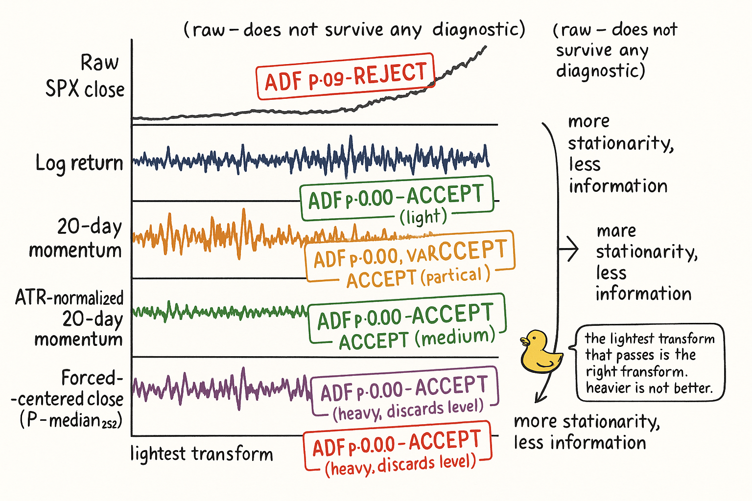
The five panels are the visual diagnostic. The same SPX data, five different feature constructions, five different stationarity verdicts. The diagnostic chooses the lightest acceptable transform, which is usually a log return alone for simple momentum and an ATR-normalized difference for price-unit features.

What this changes in practice

Three operational shifts.

Every feature carries a transform tag in the feature library. "raw_close", "log_return", "atr_norm_mom_20d", "ma_diff_10_50_atr_normalized". The tag is part of the feature's identity. Two features with the same numerator and different transforms are two different features and get logged separately.

The feature audit pipeline runs in order: construct, ADF test, coverage check, rolling-variance check, retained-MI check against a baseline log return. A feature that passes the first three but loses MI relative to the baseline log return is a heavier transform than the data required, and the lighter transform replaces it.

The cross-instrument pool is built from features whose construction makes them comparable across instruments. Log returns and ATR-normalized differences are pool-eligible by construction. Same-instrument oscillators with absolute units (MA_10 − MA_50 in price units) are not pool-eligible until they are normalized. The pool eligibility tag lives in the feature library next to the transform tag.

KEY POINTS

• Stationarizing a price-derived indicator costs information about the absolute level. The right transform is the lightest one that passes the diagnostics, not the heaviest.
• Six transforms ranked by aggressiveness: log returns, oscillators of two prices, same-bar OHLC differences, direct variance scaling, ATR-normalized differences, forced centering by rolling median.
• Log returns are the default baseline. ADF passes, coverage is near 100%, the construction absorbs proportional structure across instruments. Residual non-stationarity is variance only.
• Oscillators built from two related prices (MA_n − MA_m, or X_t − X_{t-k}) are stationary in mean by construction when the lag separation is moderate. Large lag separations fail on trending instruments.
• Same-bar OHLC differences (range, body, shadows) have structurally zero drift because both prices are recorded on the same bar. Variance still scales with price level and must be normalized separately.
• Direct variance scaling divides by a long-window rolling IQR or standard deviation. IQR is preferred when the indicator has tails. The window must be much longer than the indicator's own lookback.
• ATR normalization divides a price-unit difference by ATR over a long window. The result is unitless, comparable across instruments, and stationary in both mean and variance. The structural reason is the subject of the next article in this series.
• Forced centering by a rolling median is the heaviest transform. Use only when lighter transforms fail and the absolute level is structurally uninformative. Most "needs forced centering" indicators are poorly designed.
• Stationarize in two steps: mean first, variance second. Skipping the mean step leaves a drifting mean under stable variance. Skipping the variance step leaves volatility-regime contamination under a stable mean.
• Three look-ahead anti-patterns: full-sample z-scoring (leaks test-set statistics), centered rolling windows (leaks future bars), in-sample re-fitting of cointegration hedge ratios. Every statistic used to define a feature must be computable from data strictly before the feature's timestamp.
• On SPX 1990 to 2026, ATR-normalized 20-day momentum produces the highest retained MI (2.1 bits × 10^-3) of any tested transform, with 99% train-test coverage and ADF p = 0.00. Plain 20-day momentum has stationary mean but 78% coverage from variance drift, and forced centering passes diagnostics but discards more than half the signal of the ATR-normalized version.
• Every feature carries a transform tag and a pool-eligibility tag in the feature library. Two features with the same numerator and different transforms are different features and are logged separately.