You train an XGBoost on SPX from 1990 to 2015 with a feature set that includes raw close price, raw 50-day moving average, and raw 200-day moving average. The model produces clean in-sample numbers and a respectable 2010 to 2015 walk-forward. Cross-validated AUC: 0.531. You ship it.

The model goes live in 2016 with SPX around 2000. Through 2020 the index trades up to 3300. Through 2024 it trades up to 5800. By 2026 it sits above 6000. The feature "raw close" has been outside the maximum value the model ever saw in training for 84% of the live period. The model is extrapolating on its primary input every day.

The 2010 to 2015 walk-forward looked fine because SPX traded between 1100 and 2100 in that window, which sat inside the 1990 to 2015 training range. The walk-forward never tested the failure mode that the live deployment was guaranteed to hit. The model was not tested against the only thing that mattered: a price level outside the training support.

This article catalogs why raw price as a feature is a structural mistake. The constructive transforms that replace it (log returns, ratios, oscillators, ATR-normalized differences) belong to the next article, "How to Build Stationary Indicators from Non-Stationary Prices". The job here is to name the failure modes so a researcher rejects raw price at the feature-design stage rather than after the model breaks in production.

Three structural failures of raw price

Raw price is non-stationary in mean. SPX in 1990 averaged around 330. SPX in 2025 averages around 5500. The unconditional mean of the feature is a function of the year. A model that learned "close = 1200 is a sell signal" learned a calendar fact, not a market fact. The same calendar fact says nothing about close = 5800 in 2026 because 2026 was not in the training set.

Raw price is non-stationary in variance. The absolute dollar move per day scales with the price level. A one-percent SPX move in 1995 is 5 points. A one-percent SPX move in 2025 is 55 points. A feature like "close − close shifted 5" has a variance that grew by an order of magnitude over the sample. The model's split thresholds, distance metrics, and gradient magnitudes are all sized to the wrong variance for the live regime.

Raw price is incomparable across instruments. SPX trades at 5500. AAPL trades at 230. BTC trades at 90000. A feature defined as "close price" is not a single feature across a multi-instrument universe. It is one feature per instrument, plus an arbitrary scale factor between them. Cross-sectional models that treat raw price as a column cannot be trained at all on a pooled panel without an instrument-specific normalization, which is the same thing as not using raw price.

Raw price encodes the calendar, not the market. A model whose top feature is the price level is, by construction, a model of when the data was collected. The article "Stationarity: The Word Every Trader Ignores Until It Kills the Strategy" (forthcoming in the systems pillar) covers the broader stationarity argument. The narrow point here is that raw price fails the stationarity test by construction, not by accident.

The extrapolation trap

Three model families, three failure modes, same root cause.

Decision trees and gradient-boosted ensembles split on feature values. The split at "close ≤ 2100" partitions the training data into two non-empty leaves. The same split applied to a test set where every observation has close > 2100 sends 100% of the test data to one leaf. The model's behavior on the held-out side is the marginal prediction of that leaf, fitted on the training observations near the boundary. Outside the training support, every tree degenerates to the prediction of its nearest training leaf, regardless of whether that nearest leaf is statistically appropriate.

Neural networks with bounded activations saturate. A close-price feature normalized by the training-set mean and standard deviation produces input values around 0 to 2 for the training years and input values around 5 to 10 for the live years. Tanh and sigmoid activations saturate above 3. The network's first layer has identical activations for close = 4000 and close = 5500, because both inputs saturate at +1 after the activation. The model cannot distinguish them.

Distance-based methods (kNN, kernel regression, RBF networks) compute distances in the raw-price space. The distance from a live observation at close = 5500 to the nearest training observation at close = 2100 is 3400 in feature units. Every nearest-neighbor query in the live deployment returns the same training point (the one with the highest close), and the prediction is the local average around that training point. The model has degenerated to a constant.

Linear models extrapolate linearly. The fitted slope on "close" is determined by the in-sample relationship between price and the target. Extrapolating that slope by a factor of 3 in the live period multiplies the contribution of the feature by 3 in the model's output. If the slope was small and noisy in-sample, it dominates the prediction out-of-sample for the wrong reason. Linear models are the only family where extrapolation produces a non-constant prediction, and the non-constant prediction is the worst kind: it looks confident.

Worked example: SPX raw close versus log return

Single-feature XGBoost, SPX daily, train 1990 to 2010, test 2010 to 2026. Target y_t = sign(P_{t+1}/P_t − 1).

Two models. Model A uses raw close as the only feature. Model B uses 1-day log return ln(P_t / P_{t−1}) as the only feature. Identical hyperparameters.

Three readings.

Raw close shows a strong in-sample AUC (0.582) and a test AUC indistinguishable from a coin flip (0.498). The 8.4-point gap is the extrapolation penalty. 71% of the test rows have a raw close value larger than the maximum close seen in training. The model's splits on the raw close feature are all calibrated to a price range the test set has left behind.

Log return shows a weak in-sample AUC (0.508) and a test AUC almost identical to it (0.507). The feature has 0.4% of test rows outside the training range, which is the right-tail extreme moves from the COVID crash and the 2022 inflation regime. The model generalizes because the feature distribution is stable.

The "raw close" model is not modeling SPX. It is modeling the year. The "log return" model is weakly modeling SPX. The weak model is the honest one. The strong model is the one that broke in production.

Repeating the experiment with raw 50-day MA and raw 200-day MA reproduces the same result: large in-sample AUC, test AUC at the coin-flip line, and feature range coverage below 30%. Any feature that inherits the price level inherits the extrapolation failure.

Three diagnostics that flag a raw-price contaminated feature

Run these before the feature ships. Each one takes seconds on a daily-frequency series and rejects a feature that the backtest cannot.

ADF test on the feature itself. The augmented Dickey-Fuller test rejects the null of a unit root for stationary series and fails to reject for non-stationary series. A feature with ADF p-value above 0.05 is non-stationary at conventional levels. Raw close on SPX has ADF p ≈ 0.99 (failing to reject the unit root by construction). A 14-day RSI has ADF p ≈ 0.00. The ADF test does not distinguish between drift-stationary and trend-stationary processes for our purposes; a feature that fails ADF is rejected regardless of which non-stationarity is the cause.

Train-test feature-range coverage. Compute the fraction of test-set rows whose feature value lies within [min(feature in train), max(feature in train)]. Coverage below 95% is a structural extrapolation problem the model has no defense against. Raw close on SPX over a 20-year split has coverage around 30%. Log return over the same split has coverage near 100%. This diagnostic is independent of the model and applies to every feature regardless of its construction.

Rolling-window mean and variance drift. Compute the rolling 252-bar mean and variance of the feature across the sample. Plot both. A feature whose rolling mean drifts by more than 1 in-sample standard deviation across the sample, or whose rolling variance changes by more than a factor of 3, is non-stationary. Raw close fails both conditions on every long equity sample. Log returns fail only the variance condition during volatility regime shifts, which is the cue to apply the ATR normalization covered in the next article.

A feature passes if all three diagnostics pass. A feature fails if any one of them fails, regardless of how good its in-sample AUC looked.

When raw price appears to work and does not

Four ways raw price sneaks into the model with apparent success, all of them bias dressed as signal.

In-sample-only backtests. The train and test sets are drawn from the same overall period without a temporal split. The price level appears in both. The model learns the level. The "test" performance is a function of the calendar, not the feature.

Walk-forward windows shorter than the regime length. A 5-year training window followed by a 1-year test window keeps the price range close enough between the two that the extrapolation penalty is small per window. The cumulative walk-forward across 20 years looks fine because each individual window had near-full coverage. The model fails the moment it is deployed live and asked to extrapolate beyond the most recent training window, which by definition is the first thing live trading does.

Label leakage through normalization. Z-scoring the raw close using the full sample's mean and standard deviation, then splitting, hides the level in a feature that now looks bounded. The bound is a function of the full-sample statistics, which the live deployment does not have access to. The diagnostic: re-fit the normalization using only the training window's statistics, then re-evaluate. The performance collapse from the re-fit equals the magnitude of the leak.

Spurious common-factor effects on cointegrated pairs. A pair trade with two raw price legs can look stable because the two non-stationary series are individually non-stationary but their linear combination is stationary. The model that takes both raw prices as features cannot tell that the stationarity lives in their difference, not in either one. Replacing the two raw prices with the spread (P_1 − β P_2) is one feature instead of two and the only stationary one. The article "Stationarity: The Word Every Trader Ignores Until It Kills the Strategy" covers the cointegration case in detail.

Visualizing the extrapolation cliff

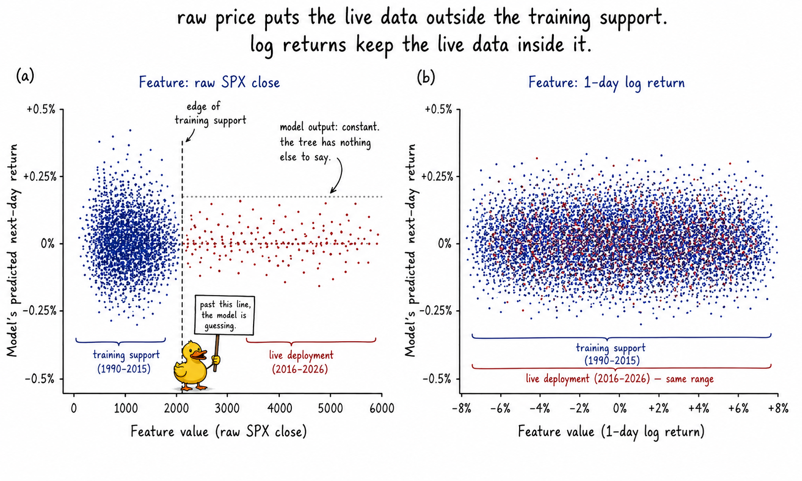
The two panels are the central diagnostic. Same underlying data, two feature constructions, two different stories about what the model is doing in production.

What can stay raw

Two narrow cases survive the case against raw price, both because the construction nets out the drift before it reaches the feature.

Same-bar OHLC differences. (high − low), (high − close), (close − low) on the same bar are not raw prices. They are differences of two prices recorded within the same one-minute or one-day window. The drift between them is structurally zero. The variance scales with the price level (a $5 range on a $20 stock is different from a $5 range on a $500 stock), so the difference must still be normalized by a volatility scale (ATR, IQR, or the bar's own midpoint). The construction is covered in the next article. The relevant point here: same-bar OHLC differences are not "raw price" in the sense this article rejects.

Cointegrated-pair spreads. P_1 − β P_2 for two cointegrated legs is stationary by construction, regardless of how non-stationary either leg is alone. The hedge ratio β must be estimated on training data and held fixed; re-fitting β on test data is the same kind of leakage that the normalization case above describes. Cointegrated spreads are an exception to the rule, not a relaxation of it.

Every other raw price feature fails for the reasons in the diagnostic section. The constructive recipe lives in the article "How to Build Stationary Indicators from Non-Stationary Prices".

What this changes in practice

Three operational shifts.

Raw close, raw OHLC, raw moving averages, and raw band envelopes (Bollinger middles, Donchian channels in price units) do not enter the feature set. The pre-modeling feature audit rejects any column whose ADF p-value is above 0.05, whose train-test coverage is below 95%, or whose rolling 252-bar mean drifts by more than one in-sample standard deviation. The audit runs before any model is trained.

Every backtest reports the train-test feature-range coverage alongside the AUC. A model whose top-importance feature has coverage below 95% is flagged in the model registry as "extrapolation-bound" and does not deploy until the feature is replaced. The walk-forward window length is sized to the regime length, not to a default of 252 bars.

Cross-instrument pooled models normalize at the feature definition, not at the model. A feature defined as "close" is not pooled across instruments. A feature defined as "1-day log return" is. The decision lives in the feature library, not in the modeling code, because the feature library is the contract that the modeling code consumes.

KEY POINTS

• Raw price is non-stationary in mean. SPX averaged 330 in 1990 and 5500 in 2025. A model trained on the 1990 distribution has no support at the 2025 distribution.
• Raw price is non-stationary in variance. The absolute dollar move per day scales with the level. Model split thresholds and gradient magnitudes calibrated to the 1990 variance are wrong for the 2025 variance by an order of magnitude.
• Raw price is incomparable across instruments. SPX at 5500 and AAPL at 230 are not on the same scale. A cross-sectional model cannot pool raw close as a column without an instrument-specific normalization, which is the same as not using raw close.
• Trees and gradient-boosted models extrapolate by sending all out-of-support observations to a single leaf. The prediction degenerates to the constant value of that leaf.
• Neural networks with bounded activations saturate beyond a few in-sample standard deviations. Distinct large values become indistinguishable post-activation.
• Distance-based methods compute distances in raw-price units. Out-of-support observations have the same nearest training neighbor (the largest training value), and the model collapses to a constant.
• Linear models extrapolate linearly. A small noisy slope multiplied by a 3× feature value in the live period dominates the prediction for the wrong reason.
• Three pre-modeling diagnostics flag raw-price contamination: ADF p-value above 0.05, train-test feature-range coverage below 95%, rolling 252-bar mean drift exceeding one in-sample standard deviation. A feature failing any one is rejected.
• A walk-forward window shorter than the regime length masks the extrapolation problem in-sample. The cumulative walk-forward looks fine because each window has near-full coverage. The live deployment fails because the first live observation extrapolates beyond the last training window.
• Z-scoring the raw close using the full sample's mean and standard deviation before splitting is label leakage. The bound is a function of statistics the live deployment cannot recompute. Re-fit normalization on training-window statistics only.
• On SPX 1990 to 2010 train and 2010 to 2026 test, a single-feature XGBoost on raw close shows in-sample AUC 0.582 and test AUC 0.498. The same model on 1-day log returns shows in-sample AUC 0.508 and test AUC 0.507. The strong in-sample model is the one that broke; the weak in-sample model is the honest one.
• Two narrow constructions can stay close to raw: same-bar OHLC differences (drift nets to zero by construction, must still be volatility-scaled) and cointegrated-pair spreads (stationary by construction, hedge ratio fixed from training). Both are exceptions, not relaxations.
• The constructive transforms that replace raw price (log returns, log differences, ATR-normalized differences, oscillators of two prices) are covered in the article "How to Build Stationary Indicators from Non-Stationary Prices"