3.1 Stationarity: The Word Every Trader Ignores Until It Kills the Strategy
Every trading rule assumes stationarity. Markets violate it constantly. Strategies do not break because the rule fails; they break because the regime moves. Rolling stats first, then ADF and KPSS.

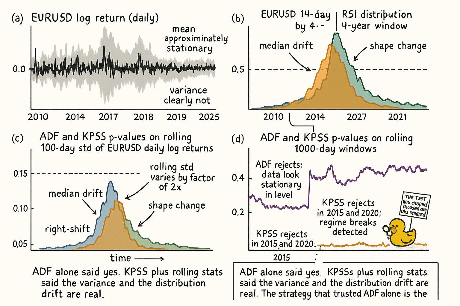
A trader builds a mean-reversion system on EURUSD daily. The rule is one line: enter long when 14-day RSI prints below 30, exit at 50, mirror short on RSI > 70 to 50. Backtest 2010 to 2014: Sharpe 1.6, max drawdown 6%, 312 round trips, profit factor 1.9. The trader ships it in January 2015. By December 2015 the system is down 14% and has not produced a single winning month since the SNB unpegged the franc. The trader assumes a parameter problem. The trader retunes RSI to 21 days and the thresholds to 25/75. The retune validates beautifully on 2010 to 2015. By mid-2016 the new version is also bleeding. The trader gives up.
The system never broke. The market it was designed for stopped existing. EURUSD daily realized volatility ran 8.4% annualized in 2010 to 2014, then climbed to 11.2% in 2015 and 9.8% in 2016, while the autocorrelation of daily returns flipped sign at the 1 to 5 day lag (mean-reverting in the first window, mildly trend-following in the second). The 14-day RSI distribution shifted: the median moved from 49.6 to 51.8, the lower 10th percentile from 24 to 27, the upper 90th from 76 to 73. None of these shifts looks dramatic on its own. Together they relocate the entire signal distribution out of the regime where the threshold rule lived. The strategy was statistically dead before the trader noticed.
This is the stationarity problem. Every trading rule, indicator, threshold, and statistical test assumes the data-generating process is stable enough across the deployment window for the in-sample statistics to be informative about the out-of-sample distribution. Markets violate this assumption almost continuously. Most violations are small enough to ignore for a year or two and then catastrophic on the third. The prior article in the publication ("Why Market Cycles Are Evanescent") established the case for one specific component (cycle period). This article generalizes the argument to every strategy component and opens Pillar 3 (Robust Systems Lab), which is the testing discipline you need once you accept that stationarity is the assumption you cannot safely take for granted.
What stationarity means operationally
A stochastic process is strictly stationary when the joint distribution of any finite collection of samples is invariant under time shifts. That definition is useless for trading because it is unverifiable from a single price path. The operational definition that matters is weak (or covariance) stationarity: the first and second moments are time-invariant.
$$ \text{Weak stationarity: } \quad \mathbb{E}[X_t] = \mu, \quad \text{Var}[X_t] = \sigma^2, \quad \text{Cov}[X_t, X_{t+k}] = \gamma(k) $$
The mean does not drift, the variance does not drift, and the autocovariance depends only on the lag k, not on the absolute time t. If those three hold, the rolling estimate of any statistic of X converges as the window grows, and a backtest computed on one slice is informative about another slice.
The stronger version (joint distribution invariance) is what predictive models silently require. A logistic regression that maps RSI to next-day return needs the joint distribution of (RSI, next-day return) to be stable. A threshold rule needs the marginal of RSI to be stable so the threshold sits at the same percentile in production as in the backtest. A volatility-targeted position-sizing rule needs the variance estimator to be unbiased. Each of these is a stationarity assumption with a different functional form.
What is non-stationary in markets
Three components, each violating stationarity in a different way.
Raw price is non-stationary in level. The mean of SPX in 2010 was 1140; in 2025 it is around 6000. The variance scales with the level (multiplicative noise). No useful statistical model takes raw price as input without first transforming it. Returns (log differences) are closer to stationary in mean (zero or near-zero unconditional mean) but the variance is still time-varying.
Volatility is non-stationary in mean and variance. Realized volatility on SPX daily moves between 8% (2017) and 35% (2008, 2020). It is mean-reverting on the 30 to 60 day horizon but the long-run mean itself drifts with the macro regime. Volatility is the most reliably non-stationary feature in markets, which is why it is the easiest one to model with explicit time-varying machinery (GARCH, HAR, regime switching) and the hardest one to ignore.
Cross-sectional structure is non-stationary in correlation. The correlation between bonds and equities was negative from 2000 to 2020, positive in 2022 and 2023, negative again in 2024. Strategies built on a fixed correlation assumption (60/40, risk parity with constant priors) carry the regime risk implicitly. Correlation is the second most non-stationary structural feature, after volatility.
Indicator distributions inherit non-stationarity from their inputs. RSI is bounded in [0, 100] but its conditional distribution given the regime is not bounded. The 90th percentile of RSI on EURUSD daily was 76 in 2010 to 2014 and 73 in 2015 to 2016. Threshold rules calibrated on one window misfire in the other. The article "Why Most Indicators Should Be Transformed Before Modeling" framed this for individual features; the present article frames it as a strategy-level concern.
Cycle structure is non-stationary in period, amplitude, and phase. The prior article ("Why Market Cycles Are Evanescent") covered this in detail.
How to test for stationarity
Three operational tests, each with different sensitivity.
Test 1: rolling mean and rolling standard deviation. Compute the mean and std on rolling 252-day windows of the feature you care about. If the rolling mean drifts by more than one rolling std across the sample, the feature is non-stationary in mean. If the rolling std varies by more than 50% across windows, the feature is non-stationary in variance. This is the cheapest, most robust diagnostic and the one most traders skip.
$$ \hat{\mu}_t = \frac{1}{W} \sum_{i=0}^{W-1} X_{t-i}, \qquad \hat{\sigma}_t = \sqrt{\frac{1}{W-1} \sum_{i=0}^{W-1} (X_{t-i} - \hat{\mu}_t)^2} $$
Test 2: Augmented Dickey-Fuller (ADF). Tests the null hypothesis that the series has a unit root (non-stationary in level). Rejecting the null at p < 0.05 is evidence that the series is stationary or trend-stationary. The test is sensitive to lag selection and weak against slow drift; passing ADF is necessary but not sufficient.
$$ \Delta X_t = \alpha + \beta t + \gamma X_{t-1} + \sum_{i=1}^{p} \delta_i \Delta X_{t-i} + \varepsilon_t $$
The null is γ = 0. Reject the null when the t-statistic on γ is more negative than the critical value (approximately −2.86 at 5% for the constant-only specification on long samples). Daily SPX log prices fail to reject (non-stationary, as expected). Daily SPX log returns reject (stationary in level). RSI on SPX daily rejects on most subsamples but the rejection is noisier than the rolling-statistic check would suggest, because ADF tests level stationarity, not distributional stationarity.
Test 3: KPSS (Kwiatkowski-Phillips-Schmidt-Shin). The complementary test: null is stationarity, alternative is non-stationarity. Use ADF and KPSS together. If ADF rejects (data look stationary) and KPSS does not reject (data look stationary), the verdict is consistent. If they disagree, the data are in the ambiguous middle, often because of slow drift. Slow drift is the topic of the next article ("Slow Wandering: The Most Dangerous Type of Market Change") and is precisely the regime where ADF/KPSS disagree.
For trading specifically, the rolling-statistic check is the most useful because the question is not "is this series mathematically stationary" (almost no market series is) but "is the violation small enough that the strategy survives." That is a magnitude question, not a hypothesis-test question.
How to make a feature more stationary
Five operational tools, each with a cost.
Tool 1: differencing. Replace X_t with ΔX_t = X_t - X_{t-1}. This removes a unit root and is the standard fix for non-stationary level. Cost: differencing destroys the level information. Differenced log price is daily log return, which is stationary in mean but the variance is still time-varying. Differencing is necessary but not sufficient.
Tool 2: log differencing (returns). Replace X_t with log(X_t) - log(X_{t-1}). For positive multiplicative processes (price, volume, volatility) this is the right transformation because the noise is multiplicative in the original scale. Most of Pillar 2's machinery operates on log returns rather than raw price for this reason.
Tool 3: ATR scaling (volatility normalization). Divide the feature by a rolling estimate of its scale.
$$ \tilde{X}_t = \frac{X_t}{\hat{\sigma}_t}, \qquad \hat{\sigma}_t = \text{ATR}(t, W) \;\text{or}\; \text{rolling std}(X, W) $$
ATR scaling makes the feature invariant to the volatility regime. A 1-ATR move in 2017 (low vol) and a 1-ATR move in 2020 (high vol) are comparable in the scaled feature. The article "Why ATR Normalization Is More Than a Volatility Trick" gave the case for this transformation in detail. Cost: scaling shrinks the dynamic range and destroys the absolute-level signal.
Tool 4: rolling normalization (z-scoring). Subtract the rolling mean and divide by the rolling std.
$$ z_t = \frac{X_t - \hat{\mu}_t}{\hat{\sigma}_t} $$
This is the strongest stationarity-forcing transformation. The rolling z-score has approximately zero mean and unit variance by construction, and the marginal distribution is approximately stable across regimes. Cost: the transformation destroys the long-run drift information that is sometimes the actual edge, and the rolling-window length W is a hyperparameter that itself overfits if chosen by backtest. The article "Rolling Normalization: Useful Tool or Hidden Overfit?" later in the pillar covers this trap.
Tool 5: rank transform (percentile normalization). Replace X_t with its rank within a rolling window, mapped to [0, 1] or [-1, 1]. The transformed feature is uniform on its rolling-window distribution by construction. Cost: ranks are insensitive to magnitude. A 1-sigma move and a 5-sigma move both end up at rank 1.0 if no other observation in the window is more extreme.
The choice between these tools is a strategy-design question, not a statistical question. The article "When Forcing Stationarity Destroys Information" later in this pillar argues the case that aggressive normalization can destroy the actual signal you wanted to trade. The right principle: apply the minimum transformation needed to keep the feature distribution stable across the regimes you expect to operate in, and verify with the rolling-statistic check rather than just trusting ADF rejection.
What this changes for backtesting
Six operational shifts. These are the framework that the rest of Pillar 3 builds on.
Shift 1: report stationarity diagnostics for every feature in the strategy. Rolling mean and std plotted across the full sample. ADF and KPSS p-values. Distribution histograms by regime. The diagnostic is the audit trail. A strategy without stationarity diagnostics is a strategy that has not been examined.
Shift 2: split backtests by regime, not by year. The convention of "2018 to 2020 in-sample, 2021 to 2023 out-of-sample" is a calendar split. The right split is by regime: low-vol vs high-vol, trend mode vs cycle mode (using the classification from "Why Market Cycles Are Evanescent"), bond-equity correlation regime, macro regime. A strategy that survives across all regimes is more robust than one that survives 2018 to 2023 with the regime-mix luck of that window.
Shift 3: walk-forward with regime-aware retraining. The article "Why Walk-Forward Testing Is Better Than One Big OOS Split" later in the pillar argues this in detail. The mechanism: retrain at quarterly cadence so the in-sample window slides across regime boundaries and the strategy adapts.
Shift 4: stress-test the strategy on synthetic non-stationary data. Generate paths with deliberate regime breaks (vol spike, mean shift, correlation flip). Measure how the strategy behaves. A strategy that drawdowns 30% on synthetic regime breaks will drawdown more on real ones. The article "Monte Carlo for Trading Systems" frames the synthetic-path machinery.
Shift 5: declare the assumed regime explicitly in the strategy spec. "This strategy assumes EURUSD daily realized vol between 6% and 10% annualized and bond-equity correlation between -0.5 and 0.0." When the assumption is violated, disable the strategy. The disable rule is part of the strategy, not a discretionary override.
Shift 6: budget for system death. The article "Why Systems Work Until They Don't" covers this. Even with stationarity diagnostics and regime-aware testing, every strategy eventually fails because the regime moves outside the training distribution. The portfolio should be sized assuming each strategy has finite life.
The slow-wandering preview
The next article in the publication ("Slow Wandering: The Most Dangerous Type of Market Change") covers the specific non-stationarity that ADF and most standard tests miss. The setup: imagine a feature whose mean drifts at 0.001 sigma per day. After 1000 days the mean has moved by one full sigma. ADF on the full sample rejects the unit root because the within-window variability dominates the drift. Rolling-mean check at 252-day window detects the drift but only after several windows have passed. The strategy backtest, computed on 5 years of data with a constant threshold, looks fine because the in-sample drift is small. The strategy fails in production once the drift accumulates past the threshold's robust range. Slow wandering is the most dangerous form of non-stationarity precisely because it does not look broken until it has already broken the strategy.
The current article frames the problem at the conceptual level. The next article frames it at the diagnostic level and gives the operational test for slow wandering. Together they are the foundation for everything else in Pillar 3.
Decision matrix
| Feature | Stationarity status | Recommended transformation | Diagnostic |
|---|---|---|---|
| Raw price (level) | Non-stationary in level | Log difference (return) | Rolling mean, ADF |
| Log returns | Stationary in mean, non-stat in variance | ATR scaling | Rolling std |
| RSI / oscillator outputs | Approximately stationary in mean, regime-dependent | Rolling normalization or rank | Rolling histogram |
| Realized volatility | Non-stationary in mean and variance | Log + rolling mean subtract | Rolling mean of log vol |
| Cross-asset correlation | Non-stationary structurally | Regime classifier as input | Rolling correlation by regime |
| Cycle period (T) | Non-stationary (covered in prior article) | Live periodogram estimate | Rolling σ_T |
| Indicator threshold | Inherits from input | Rolling percentile rank | Threshold drift over time |
The diagnostic column is the rolling-statistic check that should be on every feature before the strategy is deployed.
Anti-patterns
Five mistakes that show up when stationarity is treated as a checkbox rather than an audit.
Anti-pattern 1: "I ran ADF on the feature, it passed, the feature is stationary." ADF tests level stationarity against a unit-root null. Passing ADF rules out one specific failure mode. It does not rule out variance non-stationarity, distributional drift, or slow wandering. Combine ADF with KPSS and rolling-statistic checks before you trust the verdict.
Anti-pattern 2: "I'll fix non-stationarity with rolling normalization on a 60-bar window." Rolling normalization on a short window destroys the slow signal you might have wanted to trade. On a long window it does not adapt fast enough to regime breaks. The window length is a hyperparameter that overfits if chosen by backtest. The article "Rolling Normalization: Useful Tool or Hidden Overfit?" covers this in detail.
Anti-pattern 3: "The backtest was 5 years, that is enough." Five years of EURUSD daily covers approximately one to two macro regimes, depending on the segmentation. A strategy validated across one regime is not validated. Aim for backtests that span at least three macro regimes and report performance per regime.
Anti-pattern 4: "I differenced the price, so the input is stationary." Log returns are stationary in mean and weakly stationary in variance for short windows but exhibit strong volatility clustering and fat tails. The naive normality assumption that often follows differencing is violated. Account for the heteroskedasticity (GARCH-like models, ATR scaling) and the tail behavior (the article "Why Predictive Power Often Lives in the Tails" frames this).
Anti-pattern 5: "Stationarity does not matter, the model will figure it out." A flexible model (random forest, gradient boosting, neural network) trained on non-stationary features will capture the in-sample regime structure as if it were the true relationship. In production, when the regime shifts, the model produces confidently wrong predictions because the test distribution is now different from the training distribution. Flexibility magnifies the cost of feature non-stationarity rather than absorbing it.
Visualizing stationarity
KEY POINTS
- Every trading rule, indicator, threshold, and statistical test silently assumes the data-generating process is stationary across the deployment window. Markets violate this assumption.
- Operational stationarity is weak (covariance) stationarity: time-invariant mean, time-invariant variance, autocovariance that depends only on lag. Threshold rules, regression models, and volatility-scaled positions each invoke stationarity in a different functional form.
- Five components are the most reliably non-stationary in markets: raw price level, return variance, cross-asset correlation, indicator distributions, and cycle structure. The first four matter for every strategy; the fifth was covered in "Why Market Cycles Are Evanescent".
- The rolling-statistic check (rolling mean and std on 252-day windows) is the cheapest and most robust stationarity diagnostic. Run it before any other test.
- ADF and KPSS are complementary hypothesis tests. Use them together. Disagreement is the signature of slow drift, the topic of the next article ("Slow Wandering: The Most Dangerous Type of Market Change").
- Five tools force a feature to look more stationary: differencing, log differencing, ATR scaling, rolling z-scoring, rank transform. Each destroys some information. The right one depends on what edge the strategy is consuming.
- Five backtesting shifts follow from accepting the stationarity problem: report diagnostics per feature, split by regime not by year, walk-forward with regime-aware retraining, stress-test on synthetic non-stationary data, declare the assumed regime explicitly, and budget for system death.
- Anti-pattern: ADF passed therefore the feature is stationary. ADF rules out one failure mode. Distributional drift, variance non-stationarity, and slow wandering need other diagnostics.
- Anti-pattern: a flexible model will absorb non-stationarity. Flexible models magnify the cost of non-stationary features rather than absorbing it because they fit the in-sample regime structure as if it were the true relationship.
- The current article opens Pillar 3 (Robust Systems Lab) by establishing the structural reason that backtesting needs explicit anti-overfitting machinery: not because researchers are dishonest, but because the world is non-stationary and the assumption of stable distributions is the load-bearing assumption every trading rule depends on.
References
- Testing and Tuning Market Trading Systems - Timothy Masters (Amazon)
- Data Mining Algorithms in C++ - Timothy Masters (Amazon)
- Backtest Overfitting in the Machine Learning Era
- Predictive Value of Within-Strategy Permutation Tests for Forward Performance of Trading Rules
- Testing Strict Stationarity with Applications to Macroeconomic Time Series
- Testing Mean Stationarity of Intraday Volatility Curves
- Stationarity Analysis of the Stock Market Data and Its Application to Algorithmic Trading Strategy
- The GT-Score: A Robust Objective Function for Reducing Overfitting in Systematic Trading
- arXiv:2209.05559v6 [q-fin.ST] 31 Jan 2023
- Development of a Monte Carlo based robustness calculation and
- Stationarity tests for financial time series
- Non-Stationarity in Financial Time Series and Generic Features
- Non-stationarity and structural breaks in financial data: Challenges for valid empirical research
- Stock prices and the efficient market hypothesis: Evidence from a panel stationary test with structural breaks
- Non-stationary and stationary prediction of financial time series using machine learning methods
- Financial Time Series and Their Characteristics (Chapter excerpt from "Time Series Analysis" in a finance context)
- Time-Series Analysis | CFA Institute