3. Robust Systems Lab May 28, 2026 11 min

3.10 Rolling Normalization: Useful Tool or Hidden Overfit?

The rolling window is a hyperparameter. Picking W by IS Sharpe inflates the estimate. Pick from a structural prior matched to the strategy timescale. Audit for look-ahead. Do not retune on live P&L.

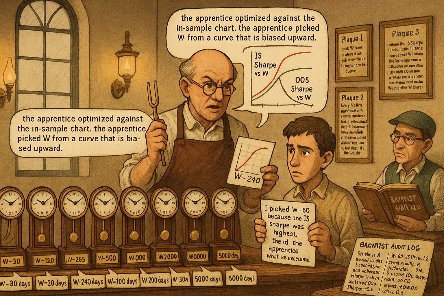
A research team builds a cross-asset trend-following strategy with a single momentum signal: 90-day return divided by an exponentially weighted moving standard deviation of returns. The team tries three values of the EWMA window: 60, 120, and 240 days. The 60-day version produces an IS Sharpe of 1.2. The 120-day version produces 1.0. The 240-day version produces 0.8. The team selects 60 days based on the IS Sharpe and ships the strategy. Live performance: Sharpe 0.4 across the next 24 months, well below all three IS estimates and well below even the worst of the three.

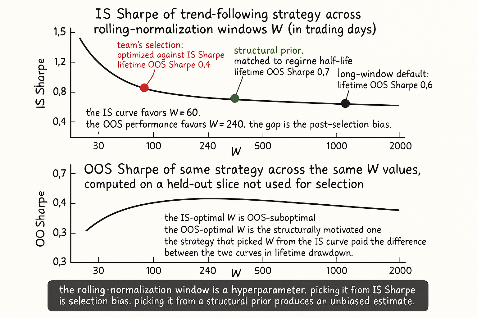
The diagnosis is not that 60 days was the wrong window in isolation. The diagnosis is that the team picked a window by optimizing against the IS Sharpe. The window is a hyperparameter, the IS comparison was an optimization, and the realized OOS performance reflects the post-selection bias. Had the team picked the 240-day window from a structural prior (matched to the regime half-life) rather than from the IS comparison, the OOS Sharpe would have been around 0.7 to 0.8, not 0.4. The optimization that looked like prudent calibration was an overfit on the rolling-window length itself. This article covers the trap and the operational defenses against it.

The article "How to Make Indicators More Stationary" gave rolling normalization as one of several tools. The article "When Forcing Stationarity Destroys Information" gave the case where the tool destroys signal. This article covers the more subtle failure mode where the tool is appropriate for the strategy and the parameter (the window length) silently becomes the overfitting hyperparameter. Most production rolling-normalization implementations have this problem to some degree; the question is how much, and what discipline reduces the cost.

The mechanics of rolling normalization

The standard form. At each time t, compute the rolling mean and rolling standard deviation of a feature X over the past W observations, then standardize the current value.

$$ z_t = \frac{X_t - \hat{\mu}_t^{(W)}}{\hat{\sigma}_t^{(W)}}, \qquad \hat{\mu}_t^{(W)} = \frac{1}{W} \sum_{i=1}^{W} X_{t-i}, \quad \hat{\sigma}_t^{(W)} = \sqrt{\frac{1}{W-1} \sum_{i=1}^{W} (X_{t-i} - \hat{\mu}_t^{(W)})^2} $$

The rolling rank is the percentile-based variant. Rolling z-score is the moment-based variant. Both transform a feature whose unconditional distribution is non-stationary into a feature whose within-window distribution is approximately uniform (rank) or approximately N(0,1) (z-score). The transformation matters when the strategy threshold rule needs the input distribution to be stable.

The hidden parameter is W. Different choices of W produce different transformed features. The transformed feature is a different feature for each W, with different predictive properties, different stationarity profiles, and different OOS behavior. The phrase "the same feature with a different window" misdescribes the operation.

The window-length trade-off

Three structural properties move with W in opposite directions.

Property 1: regime-tracking speed. A short W (e.g., 30 to 60 days) tracks regime changes quickly. The transformed feature responds to a vol regime shift within weeks. A long W (e.g., 1000+ days) tracks regime changes slowly; the transformed feature lags the regime shift by months.

Property 2: signal preservation. A short W eats slow drift in the underlying signal. If the strategy depends on a multi-year cross-sectional momentum, a 60-day rolling z-score within each asset removes precisely the signal (the example in "When Forcing Stationarity Destroys Information"). A long W preserves slow drift.

Property 3: estimation precision. A short W produces noisy estimates of mean and std. A long W produces precise estimates. The standard error of the rolling z-score scales with 1/sqrt(W) in the noise component.

$$ \text{SE}(z_t) \approx \sqrt{\frac{1}{W} \cdot \left(1 + \frac{z_t^2}{2}\right)} $$

The operational consequence: there is no globally correct W. The right choice depends on whether the strategy needs fast regime tracking (short W is right), or signal preservation (long W is right), or estimation precision (longer is generally better). Different strategies in the same portfolio may need different W values for the same underlying feature. A unified W "for all features in the strategy" is a reasonable default but a structural compromise.

The optimization-against-the-backtest trap

The empirical pattern from the opening example. The researcher tries multiple W values and picks the one with the highest IS Sharpe. The trap has three failure modes that compound.

Failure 1: in-sample noise. The IS Sharpe at each W has its own standard error. A Sharpe of 1.2 for W=60 versus 1.0 for W=120 may not be a meaningful difference; it may be sampling noise. The researcher who picks the higher one is selecting on noise rather than on edge.

Failure 2: lookback selection bias. The set of W values tried is itself an information leakage. If the researcher tried W = 30, 60, 90, 120, 180, 240, 365, 500, 1000 and picked the best, the implicit search width is much larger than three values. The right inference accounts for the search width across all considered Ws, not the chosen one alone.

Failure 3: the overfit grows with the granularity. Trying W = 60, 65, 70, 75, ..., 240 gives 37 candidates. The IS Sharpe of the best of 37 is higher than the IS Sharpe of any one structural choice, with the gap reflecting search luck rather than edge. The article "Why More Parameters Make a Strategy Easier to Sell and Easier to Break" framed the general degrees-of-freedom concern; rolling normalization windows fall within that concern.

Causality and look-ahead

Two specific look-ahead patterns to audit.

Pattern 1: full-sample normalization. Some implementations compute the mean and std on the entire sample, then apply the standardization point-by-point. The implementation is fast and produces a clean-looking transformed series. The implementation is also look-ahead biased: the mean and std at time t use observations from t+1, t+2, ..., T. The OOS estimate that depends on full-sample normalization will not generalize because the live trading version cannot use future observations to compute the historical mean.

Pattern 2: warm-up period filled with the first valid value. The rolling estimate is undefined for the first W observations. Some implementations fill these with the first valid rolling estimate (backfilling the warm-up with the W+1-th value). The backfill is a soft form of look-ahead because the W+1-th value uses observations 1 through W+1, but the strategy is then allowed to trade on observations 1 through W using the backfilled estimate. The standard fix: do not trade during the warm-up. Live trading does not generate the warm-up issue because the strategy starts after sufficient history; backtests need to drop the warm-up window.

Pattern 3: shifted rolling estimates that include the current observation. The rolling estimate at t should be computed from observations t-1, t-2, ..., t-W. Some implementations include t in the rolling window (using observations t, t-1, ..., t-W+1). Including t means the standardization at t uses information from t itself, which is an instantaneous-information leakage. The standardized value at t is a function of X_t which includes the current observation; the test that the standardized z_t predicts the next return is contaminated by the contemporaneous coupling.

Each of these patterns can be present without the researcher noticing, with code paths that use vectorized libraries the common offender. The article "Why OOS Failure Is Often a Stationarity Failure" framed the leakage detection step. Run the audit on every rolling-normalization implementation before trusting the results.

Choosing W without optimization

Five operational rules.

Rule 1: pick W from a structural prior, not from the IS Sharpe. The structural prior is set by the strategy's intended timescale. A strategy that holds positions for 5 days needs a W that is much longer than 5 days (so the rolling window does not see only the holding period). A strategy that targets a specific regime timescale (e.g., the macro cycle, approximately 5 to 7 years) needs W matched to that timescale. The article "How to Make Indicators More Stationary" gave the timescale-matching guideline.

Rule 2: pick W once and document the choice. The choice is part of the strategy specification. Subsequent retraining or recalibration uses the same W. Changing W in production is a methodology change that requires the same rigor as the original deployment.

Rule 3: report the strategy's IS performance across multiple W values, beyond the chosen one alone. The robustness check: if the strategy's Sharpe varies across a wide range over W = 100, 252, 500, 1000, the result is fragile and the strategy is not robust to the rolling-window choice. If the Sharpe is approximately constant across the range, the choice is non-critical and the strategy is robust.

Rule 4: avoid the "we will retune W if the strategy underperforms" trap. Retuning W in response to underperformance is a discretionary override of the original calibration and is a common form of look-ahead bias in live trading. The strategy specification should set W at deployment and the operational protocol should not allow W to be changed in response to OOS performance.

Rule 5: when the IS Sharpe is very sensitive to W, treat the sensitivity as a signal that the strategy is overfit to a specific regime. A robust strategy is approximately insensitive to small changes in W. A strategy that drops from Sharpe 1.2 at W=60 to Sharpe 0.5 at W=120 is overfit to the W=60 regime structure, regardless of which W is "correct".

Rolling normalization done right

Three checks that confirm the tool is appropriate.

Check 1: the underlying feature has a non-stationary distribution that is uncorrelated with the strategy's signal axis. The feature has slow drift in mean and variance that the strategy does not depend on for its edge. Rolling normalization removes the drift without removing the signal.

Check 2: the strategy uses the feature as an input to a threshold rule whose threshold is fixed in standardized units. The standardized feature has a stable distribution by construction, so the threshold has consistent operational meaning across regimes.

Check 3: the strategy's signal lives in the high-frequency component of the feature, not in the slow drift. Rolling normalization is a high-pass filter on the feature; the strategy that consumes high-frequency variation benefits from the filtering.

If any of the three checks fails, the tool is wrong for the strategy. If check 1 fails, rolling normalization eats the drift that was the signal; use cross-sectional or regime-conditional methods instead. If check 2 fails, the threshold rule is not fixed in standardized units and the standardization adds noise; consider rank-based or quantile-based thresholds. If check 3 fails, rolling normalization removes the slow drift that the strategy needs; do not apply the transformation, or apply it with a much longer W.

Anti-patterns

Five mistakes specific to rolling normalization.

Anti-pattern 1: the W-grid search. Trying W = 30, 60, 90, ..., 1000 and picking the best IS Sharpe is overfitting. The right discipline is structural prior + insensitivity check.

Anti-pattern 2: the implicit W-search through "robustness analysis". Reporting "the strategy works for W from 60 to 240 with Sharpe between 0.9 and 1.2" is itself a search over six values; the post-search Sharpe distribution is biased. Report the IS Sharpe at the structurally chosen W; do robustness checks on a separate validation slice.

Anti-pattern 3: full-sample normalization for "convenience". The convenience is that the implementation is faster and the rolling-estimate noise is lower. The cost is look-ahead bias. The convenience is not worth the bias.

Anti-pattern 4: changing W in response to live underperformance. The retune is a soft form of overfitting because it incorporates live performance into the training. The strategy specification should set W at deployment; live underperformance triggers the decommission protocol from "How to Detect When a Trading System Is Dying", not a recalibration of W.

Anti-pattern 5: assuming the strategy is robust to W on the grounds that the IS Sharpe is similar across two values. Two W values, both picked from a search, can be near-equivalent in IS and very different in OOS. The robustness check needs to use values that span the structural range and were not part of the original search.

Decision matrix

Strategy timescale	Strategy goal	Recommended W	Verification
Intraday	Signal lives in minutes-to-hours	30 to 60 minutes (within-day rolling)	Stable distribution within typical day
Multi-day swing	Signal lives in days-to-weeks	60 to 250 trading days	Histograms by month equal
Multi-month trend	Signal lives in months	500 to 1000 trading days	Histograms by year equal
Multi-year factor	Signal lives in years	2500+ trading days or full sample (passive)	Histograms by 5-year window equal
Vol regime detection	Regime classification	60 to 250 trading days with hysteresis	Rolling stat stable, transitions visible
Cross-sectional comparison	Universe-relative	Use cross-sectional norm, not time-series	Cross-sectional rank stable per date
Spread / pairs	Within-pair mean reversion	Match to half-life of mean reversion	Half-life test from Pillar 2
Macro cycle	Cycle-conditional positioning	1000 to 2500 trading days	Within-cycle distribution stable

The matrix matches W to strategy timescale rather than to backtest performance. The discipline: pick from the matrix, document the choice, run the insensitivity check, do not optimize.

Visualizing the W trap

KEY POINTS

Rolling normalization (z-score or rank within a rolling W-bar window) is a useful tool for stationarizing a feature whose unconditional distribution drifts. The window length W is a hyperparameter and the most common source of overfitting in this part of the pipeline.
Three structural properties move with W in opposite directions: regime-tracking speed (short W is faster), signal preservation (long W preserves slow drift), estimation precision (long W is more precise). There is no globally correct W; the right choice depends on the strategy.
The optimization-against-backtest trap. Picking W by maximizing IS Sharpe inflates the in-sample estimate by an amount that scales with the search width. The resulting OOS Sharpe is materially lower than the IS Sharpe.
Three look-ahead patterns to audit: full-sample normalization (uses the whole sample's mean and std), warm-up period backfilled with first valid value, shifted rolling estimates that include the current observation. Each contaminates the backtest.
Five operational rules for choosing W: pick from a structural prior matched to the strategy's intended timescale, document the choice in the strategy spec, report performance across multiple W values for robustness, do not retune W in response to live underperformance, treat W-sensitivity as a sign of overfitting to a specific regime.
Three checks that confirm rolling normalization is the right tool: feature non-stationarity is uncorrelated with the strategy's signal axis, threshold rule is in standardized units, signal lives in the high-frequency component.
Anti-pattern: the W-grid search across 30 to 1000 with selection on best IS Sharpe. Anti-pattern: the implicit W-search through "robustness analysis". Anti-pattern: full-sample normalization for convenience. Anti-pattern: changing W in response to live underperformance. Anti-pattern: assuming W-robustness from a small IS comparison.
The right discipline matches W to strategy timescale: intraday signal gets minutes to hours, multi-day swing gets 60 to 250 trading days, multi-month trend gets 500 to 1000, multi-year factor gets 2500+ or full-sample-passive, vol regime detection gets 60 to 250 with hysteresis.
Cross-sectional strategies use cross-sectional normalization, not time-series rolling normalization. The article "When Forcing Stationarity Destroys Information" framed this distinction; the present article gives the operational rule.
The current article gives the rolling-normalization-specific discipline. The next article in the publication ("Regime Coverage: Why Your Backtest Needs Different Market States") covers the upstream question that often drives the W choice: how to ensure the backtest covers enough regimes that the W choice is validated against the right distribution of conditions.