3. Robust Systems Lab May 28, 2026 11 min

3.11 Regime Coverage: Why Your Backtest Needs Different Market States

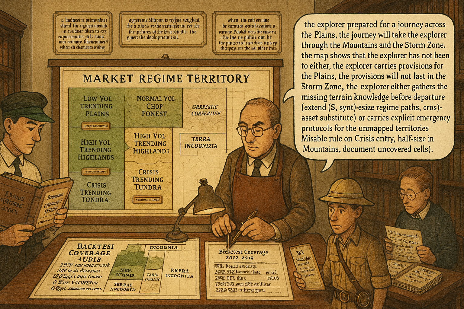
A backtest is informative about regimes it covers, silent about the rest. Stratify by vol, trend, correlation, macro, microstructure. Report cell Sharpe with CI. Ship when every required cell passes.

A research desk completes a backtest of a US equity beta-neutral pairs strategy on the period January 2010 to December 2019. The backtest reports Sharpe 1.6, max drawdown 7%, 1850 round-trip trades, profit factor 1.7, win rate 56%. The desk ships the strategy in January 2020. Live performance from 2020 to 2024: Sharpe 0.3, max drawdown 22%, profit factor 1.1. The desk's first instinct is the same diagnostic flow covered in "Why OOS Failure Is Often a Stationarity Failure": run permutation tests, audit the pipeline, check the sample size, run the regime overlap KS test on the IS-vs-OOS feature distributions. The KS test rejects equality on multiple features at p < 0.001. The diagnosis is regime mismatch.

The deeper question is upstream of the diagnosis. The backtest period (2010 to 2019) was a single macro regime: post-GFC recovery, persistent QE, low and falling interest rates, low and falling realized volatility, dominant equity beta as the cross-sectional risk factor. The regime was unusually stable for an unusually long time. The backtest was informative about that regime. The backtest was not informative about any other regime, because no other regime was in the sample. The strategy that the backtest validated is a strategy that works in 2010-to-2019 conditions; it is not a strategy that works in 2020-to-2024 conditions, and the backtest gave no information about the latter.

The discipline that prevents this failure is regime coverage: the requirement that the backtest sample contains enough trading days in each of the regimes the strategy will face in deployment. The article "Why OOS Failure Is Often a Stationarity Failure" framed regime coverage as the proper denominator for OOS validation. The articles "Volatility Regimes and Strategy Survival" and "Why Volatility Is More Non-Stationary Than Trend" framed the specific case of vol regime coverage. This article gives the operational machinery: how to enumerate the regimes that matter, how to verify coverage in the IS sample, how to report stratified performance, how to handle rare regimes through synthesis, and how to decide whether the strategy is deployment-ready or whether more data (or synthetic data) is needed.

Enumerating the regime axes

Five regime axes that matter for most strategies. The exact set depends on the strategy class.

Axis 1: realized volatility. Three to four bins (low, normal, high, crisis), thresholded against the asset's own historical distribution. Covered in "Volatility Regimes and Strategy Survival".

Axis 2: trend versus chop. Two to three bins by autocorrelation of returns at the relevant horizon, or by the absolute t-statistic of the rolling mean return. A strategy that bets on direction needs trending bins; a strategy that bets on mean reversion needs chop bins.

Axis 3: cross-asset correlation regime. Two to three bins by rolling correlation of the strategy's primary asset to other reference assets (SPX, AGG, USD, gold). Strategies that consume correlation structure need each regime represented.

Axis 4: macro regime. Two to four bins by macro state (recession vs expansion, inflation regime, monetary-policy stance). Macro-conditional strategies need each macro regime represented in IS.

Axis 5: microstructure era. The structural state of the market: pre-decimalization, decimalization era, HFT era, post-Reg-NMS, post-2010 ETF dominance, post-2020 retail-flow regime. For high-frequency or microstructure-sensitive strategies, the era boundary is the regime boundary.

A two-axis stratification (e.g., vol-by-trend) gives 6 to 9 regime cells. A three-axis stratification gives 12 to 27. The minimum requirement: for each cell that the live deployment will face, the IS sample contains at least N trading days (typically 252 days as a minimum for crude estimates, 1000 for confident estimates).

Computing the regime distribution of the IS sample

Three steps.

Step 1: classify each IS day into a regime cell. For the SPX example: each day is classified as (vol regime in {low, normal, high, crisis}) x (trend mode in {trend, chop}) using the thresholds from prior articles. Each day gets a tuple label.

Step 2: count the IS days per cell.

$$ N_c^{(\text{IS})} = \#\{t \in \text{IS sample} : \text{regime}(t) = c\}, \qquad \forall c \in \mathcal{C} $$

Step 3: compare the IS regime distribution to the historical or expected long-run regime distribution.

$$ p_c^{(\text{IS})} = \frac{N_c^{(\text{IS})}}{|\text{IS sample}|}, \qquad p_c^{(\text{long-run})} = \frac{N_c^{(\text{long-run})}}{|\text{long-run sample}|} $$

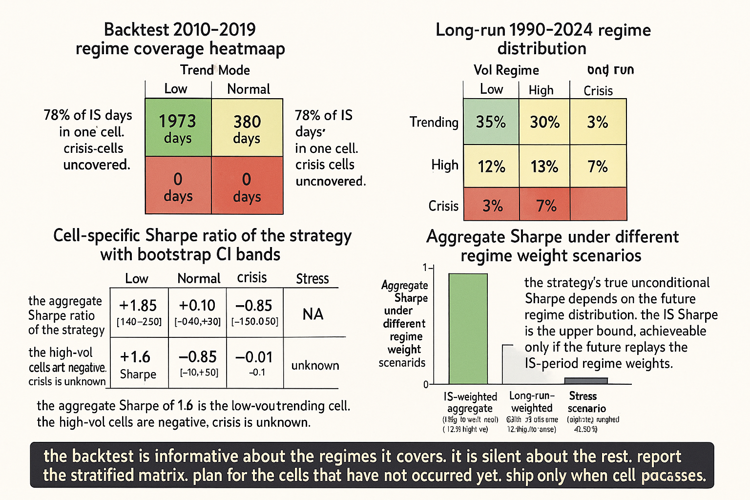
A material difference between the two distributions (e.g., IS p_crisis = 0.005 versus long-run p_crisis = 0.03) is the signature of an unrepresentative IS sample. The 2010 to 2019 SPX example: the IS distribution had p_low_vol_trending = 0.78, p_normal_vol_chop = 0.15, p_high_vol = 0.05, p_crisis = 0.0. The long-run distribution (1990 to 2024) had p_low_vol_trending = 0.40, p_normal_vol_chop = 0.30, p_high_vol = 0.25, p_crisis = 0.05. The IS sample concentrated 78% of trading days in one regime cell; that cell carries 78% of the IS Sharpe estimate, and the strategy was implicitly tuned for that one cell.

Stratified Sharpe reporting

The regime-stratified report. For each cell with N >= 252 days, compute the cell-specific Sharpe with its bootstrap confidence band. Report the matrix.

$$ \text{SR}_c = \frac{\bar{r}_c}{\hat{\sigma}_c} \cdot \sqrt{252}, \qquad \text{CI}(\text{SR}_c) = \pm \frac{2}{\sqrt{N_c / 252}} $$

The aggregate IS Sharpe is the regime-weighted average of cell Sharpes. The right reporting:

$$ \begin{array}{l|c|c|c} \text{Regime cell} & \text{Days in IS} & \text{Cell Sharpe} & \text{Cell CI} \\ \hline \text{Low vol, trending} & 1973 & +1.85 & [+1.40, +2.30] \\ \text{Normal vol, chop} & 380 & +0.10 & [-0.40, +0.60] \\ \text{High vol} & 130 & -0.85 & [-2.20, +0.50] \\ \text{Crisis} & 0 & \text{N/A} & \text{insufficient data} \\ \end{array} $$

The aggregate IS Sharpe of 1.6 is dominated by the low-vol-trending cell (1973 days at Sharpe 1.85). The strategy is a low-vol-trending strategy in operational terms, with a near-zero contribution from the chop cell and a negative contribution from the high-vol cell. The crisis cell is uncovered. The aggregate number hides the fragility.

The stratified report transforms the deployment decision. Without it, the desk sees Sharpe 1.6 and ships. With it, the desk sees that 78% of the IS sample is in one regime, the strategy is negative in another regime, and a key regime (crisis) has zero coverage. The conclusion: this strategy is not deployment-ready until either more data is collected (waiting for natural regime variation) or the missing regimes are covered through synthesis or alternative samples.

Handling rare regimes

Three approaches when the IS sample does not cover a key regime.

Approach 1: extend the IS sample backward. The standard fix: pull historical data further back to capture more regime variation. The 2010-2019 SPX backtest extended to 1990-2019 covers the 2000-2002 dot-com regime, the 2008 GFC, and several intermediate regimes. The cost: the long history may include microstructure or macro eras that no longer apply. The 1990s pre-decimalization SPX is a different microstructure than the 2024 SPX. Decide which historical regimes are representative of the current era and which are not.

Approach 2: synthesize regime-specific paths. Generate synthetic price paths that have the statistical properties of each missing regime (vol level, autocorrelation, return distribution, cross-asset correlation). Backtest the strategy on the synthetic paths. The synthetic Sharpe is informative about how the strategy would perform if the missing regime occurred. The article "Monte Carlo for Trading Systems" later in this pillar covers the synthesis machinery in detail.

Approach 3: cross-asset / cross-instrument substitution. If SPX 2010-2019 covers only one regime, look at other equity indices, other countries, or other asset classes during the same period for analog regimes. The Nikkei 1990-2019 covers high-vol-deflationary regimes that SPX does not. Substituting a comparable regime from a different instrument provides a noisy estimate of how the strategy would have behaved in that regime on SPX.

Each approach has costs. Backward extension may include irrelevant eras. Synthesis assumes a parametric model of the regime that may be wrong. Cross-asset substitution assumes the strategy generalizes across instruments. Use multiple approaches in parallel and report each separately; the agreement (or disagreement) between approaches is itself informative.

The deployment decision rule

A simple rule that makes regime coverage operational.

$$ \text{Deploy} \iff \forall c \in \mathcal{C}_{\text{required}}: \; N_c^{(\text{IS or synthetic})} \ge N_{\min} \text{ AND } \text{SR}_c \ge \text{SR}_{\min} $$

The rule has two conditions. First, every required regime cell must have at least N_min days of coverage (in IS or in synthesized data). Second, the cell-specific Sharpe must exceed SR_min in every required cell. A strategy that earns positive returns in three out of four cells but is severely negative in the fourth is not deployment-ready: the negative cell will produce drawdowns proportional to its prevalence in the live deployment.

Typical thresholds: N_min = 252 days per cell (one year of representative trading days), SR_min = 0.0 (the strategy must at least break even in each cell, ideally positive). Stricter thresholds for high-stakes deployment: N_min = 1000, SR_min = 0.3. The thresholds are operational defaults, not laws of nature; calibrate to the strategy's risk budget and the team's tolerance for regime-conditional losses.

Cases of impossible regime coverage

Some regimes do not have enough historical instances to support a sample-size-adequate backtest. SPX crisis regimes (>30% annualized vol) constitute approximately 3% of days across 1990-2024, with the largest events clustered in 2008 and 2020. A strategy needs more than three or four crisis events to claim it is robust to crises; the historical record does not provide that many independent events.

The honest acknowledgment: certain strategies cannot be fully validated against historical regime coverage because the regime is too rare. The right response: explicitly document the uncovered regime in the strategy specification, size the strategy assuming the uncovered regime will occur, and have a written disable rule for when the live data enters the uncovered regime. The article "Why Systems Work Until They Don't" framed the finite-life-budgeting approach; uncovered regimes are one specific case where the budgeting needs to be more conservative.

Anti-patterns

Five mistakes specific to regime coverage.

Anti-pattern 1: the convenient backtest window. Picking 2010-2019 as the backtest period because the data is clean and the volatility is low produces a backtest that validates one regime. The convenience is also the bias. The article "Why OOS Failure Is Often a Stationarity Failure" framed this in terms of OOS calendar selection; the same point applies to IS calendar selection.

Anti-pattern 2: the aggregate-Sharpe-as-validation report. Reporting only the aggregate IS Sharpe without the stratified cell breakdown is not informative about the strategy's regime sensitivity. The aggregate hides the fragility. The right report is always stratified.

Anti-pattern 3: assuming "the next decade will look like the last decade". The post-GFC SPX 2010-2019 was a single-regime decade. The post-2020 SPX has been a multi-regime period. Strategies validated on 2010-2019 implicitly assumed regime persistence and paid the cost when the regime changed. Plan for regime changes; do not assume continuity.

Anti-pattern 4: synthesizing without acknowledgment. Some shops generate synthetic data to cover gaps but report the synthetic-augmented Sharpe as if it were a historical Sharpe. The synthesis is a parametric model assumption that may be wrong; the synthetic Sharpe should always be reported separately from the historical Sharpe.

Anti-pattern 5: skipping the regime coverage check. The desk runs the backtest, sees a high Sharpe, and ships. The regime coverage check would have shown that the high Sharpe is from one regime cell that may not persist. The skipped check is the upstream cause of the OOS failure that the desk later misdiagnoses as overfitting.

Decision matrix

IS regime coverage	Deploy decision	Action
All required cells, all positive Sharpe, all N >= 252	Deploy	Standard production protocol
All cells covered but one negative Sharpe	Deploy with cell gating	Disable in negative-Sharpe regime per "Volatility Regimes and Strategy Survival"
Some cells under-covered (N < 100) but positive	Deploy at reduced size	Half allocation, monitor regime entry
Some cells uncovered (N = 0)	Do not deploy	Extend IS sample, synthesize, or substitute
Aggregate Sharpe high but driven by one cell (>70% of days)	Do not deploy	Strategy is single-regime; reframe accordingly
Synthetic-augmented coverage shows positive Sharpe per cell	Conditional deploy	Document synthesis assumptions in spec, monitor real regime entry
Crisis cell uncovered, no synthesis	Deploy with hard disable rule	Decommission on crisis entry per "How to Detect When a Trading System Is Dying"

The matrix is operational. The key principle: a backtest is informative about the regimes it covers and silent about the rest. The deployment decision is the question of whether the live regime distribution will match the IS regime distribution well enough for the IS Sharpe to be predictive.

Visualizing regime coverage

KEY POINTS

A backtest is informative about the regimes its sample covers and silent about regimes it does not. The 2010-2019 SPX backtest covers one regime well and most other regimes barely or not at all. Strategies validated on this sample are validated for that regime, not for all regimes.
Five regime axes matter for most strategies: realized volatility, trend versus chop, cross-asset correlation, macro regime, microstructure era. A two-axis stratification gives 6 to 9 cells; a three-axis stratification gives 12 to 27.
Regime coverage check: classify each IS day into a regime cell, count days per cell, compare to the long-run or expected distribution. Material under-coverage of any cell is the signature of a regime-biased IS sample.
Stratified Sharpe report: cell-specific Sharpe with bootstrap confidence bands, plus the cell's count of IS days. The aggregate IS Sharpe is the regime-weighted average and is dominated by the most-represented cell.
The 2010-2019 SPX example: aggregate IS Sharpe 1.6, dominated by low-vol-trending (1973 days at Sharpe 1.85). Other cells are near-zero or negative. Crisis cells are uncovered. The aggregate hides the fragility.
Three approaches to handle rare or uncovered regimes: extend the IS sample backward (cost: includes irrelevant historical eras), synthesize regime-specific paths (cost: parametric model assumption), cross-asset substitution (cost: assumes generalization across instruments). Use multiple approaches and report each separately.
Deployment decision rule: every required regime cell must have N >= N_min days of coverage (in IS or synthesized) AND cell-specific Sharpe must be at least SR_min. Typical defaults: N_min = 252, SR_min = 0.0. Stricter for high-stakes: N_min = 1000, SR_min = 0.3.
When a regime cannot be covered (e.g., crisis events too rare for meaningful backtest), explicitly document the uncovered regime, size the strategy assuming it will occur, write a disable rule for live entry into the uncovered regime.
Anti-pattern: the convenient backtest window (2010-2019 SPX). Convenience is also bias. Anti-pattern: aggregate-Sharpe-as-validation. The aggregate hides fragility. Anti-pattern: assuming the next decade resembles the last. Anti-pattern: synthesizing without acknowledgment. Anti-pattern: skipping the regime coverage check.
The current article gives the regime-coverage discipline that the rest of Pillar 3 (walk-forward, Monte Carlo, CSCV, parameter stability, stop-loss analysis, profit-factor critique) all depend on. A strategy that passes those tests on a single-regime sample is not validated. The next article in the publication ("The Difference Between Robustness and Optimization") frames the upstream principle that regime coverage is a property of the testing process, not of the optimization process.