3. Robust Systems Lab May 28, 2026 10 min

3.24 Why Walk-Forward Testing Is Better Than One Big OOS Split

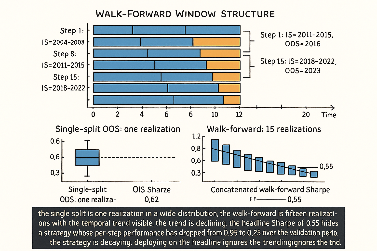
Walk-forward chains many IS-OOS pairs, producing many OOS realizations and a temporal trend. A single split is one realization. Read the per-step distribution and trend, not the headline alone.

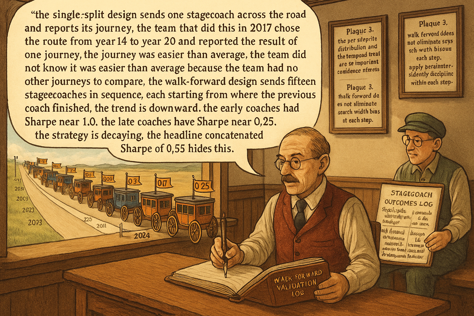
A team validates a strategy using a 70-30 split: 14 years of IS (2004-2017), 6 years of OOS (2018-2023). The IS Sharpe is 0.95 with the optimized parameters. The OOS Sharpe is 0.62. The team interprets the OOS as confirmation: "the strategy generalizes, OOS Sharpe is positive by a margin, deploy". The strategy ships in 2024 and produces a Sharpe of approximately 0.15 in the first year.

The post-mortem reveals the problem with the single-split design. The 6-year OOS window happened to span 2018-2023, which included a benign equity environment with a brief 2020 disruption that recovered quickly and a 2022 drawdown that the strategy navigated reasonably. The OOS Sharpe of 0.62 was one realization of the strategy's performance; if the OOS had been 2008-2013 (financial-crisis aftermath), the realization would have been different. If the OOS had been 1999-2004 (dot-com bust), different again. The team had no way to know which OOS realization was representative because they had only one. The single-split design produces a single OOS Sharpe number, and the team treats it as the OOS estimate, when it is one draw from a wide distribution of possible OOS outcomes.

Walk-forward testing produces many such draws. The procedure: divide the data into multiple consecutive IS-OOS pairs, each shorter than the single-split design. For each pair, optimize on the IS portion, evaluate on the OOS portion, then roll the window forward and repeat. The result is a sequence of OOS Sharpes, one per walk-forward step, that approximates the strategy's performance under the cadence at which it would be redeployed. The article "CSCV: A Direct Probability of Backtest Overfit" gave a combinatorial alternative; this article covers the time-respecting alternative that simulates real-time deployment. Both reduce the variance of the OOS estimate compared to the single-split design; walk-forward additionally captures the temporal dynamics of strategy decay and adaptation.

Walk-forward testing, mechanics

Five steps with concrete numbers.

Step 1: choose the in-sample window length and the out-of-sample window length. Common choices: IS = 3 years, OOS = 6 months. Or IS = 5 years, OOS = 1 year. The IS window must be long enough to support meaningful parameter optimization (typically 100+ effective trades; the article "Trade-Count Thresholds for Backtest Reliability" framed the threshold). The OOS window must be long enough to produce a meaningful Sharpe estimate per step (typically 30+ trades, with the standard-error-of-Sharpe interpretation from the same article).

Step 2: anchored or rolling. Anchored walk-forward keeps the IS window starting at the same date and grows it; the IS window at step k is from date 0 to date k * OOS_length. Rolling walk-forward keeps the IS window length fixed; the IS window slides forward at each step. Rolling is more responsive to drift but uses less data per step. Anchored uses more data but is slower to adapt. For most strategies, rolling with a 3-5 year IS is the operational standard.

Step 3: at each step, optimize on IS and run on OOS. The optimization uses whatever discipline the article "The Difference Between Robustness and Optimization" framed (parameter-stability mapping, plateau selection, structural-prior anchoring). The OOS evaluation uses the chosen parameters with no further adjustment. The OOS Sharpe is recorded.

Step 4: roll the window forward by OOS_length. With OOS = 6 months, the window advances 6 months. The next IS window now includes the previous OOS period (or, for rolling, the IS shifts forward 6 months).

Step 5: aggregate the results. The walk-forward Sharpe is computed from the concatenated OOS returns across all steps, not from the average of the per-step Sharpes. The walk-forward Sharpe is one number; the per-step Sharpes are the diagnostic distribution.

For 20 years of data with IS = 5 years and OOS = 1 year (rolling), the walk-forward produces 15 IS-OOS pairs (the first IS uses years 0-5, the first OOS is year 5; the next IS uses years 1-6, the next OOS is year 6; etc.). The 15 OOS Sharpes are the per-step distribution; the concatenated 15-year OOS return series produces the walk-forward Sharpe.

Walk-forward's additions over single-split

Four diagnostic outputs.

Output 1: per-step Sharpe distribution. The 15 per-step Sharpes are 15 realizations of the OOS Sharpe. The mean and standard deviation of the 15 give a confidence interval that is much tighter than the standard error of a single OOS Sharpe. The article "Trade-Count Thresholds for Backtest Reliability" gave the single-OOS-Sharpe SE; the walk-forward SE is approximately the single-step SE divided by sqrt(15), assuming the per-step Sharpes are approximately independent.

$$ \text{SE}(\overline{\text{SR}}_{\text{WF}}) \approx \frac{\text{SE}(\text{SR}_{\text{single OOS}})}{\sqrt{N_{\text{steps}}}} $$

Output 2: temporal trend in performance. If the per-step Sharpes decline monotonically across the walk-forward sequence, the strategy is decaying. The article "Why Systems Work Until They Don't" framed the four mechanisms; the walk-forward trend visualization detects the decay before deployment. A flat per-step distribution is consistent with stable performance; a declining distribution is a deployment red flag.

Output 3: regime-conditional behavior. The per-step Sharpes can be cross-tabulated with the regime classification of each OOS window (bull/bear, low-vol/high-vol, etc.). The article "Regime Coverage: Why Your Backtest Needs Different Market States" framed the regime stratification; walk-forward composes with it because each step has a known calendar period and the regime of that period is known.

Output 4: parameter-stability over time. The optimized parameters at each walk-forward step can be compared. If the parameters change across a wide range from step to step (e.g., the optimal lookback wanders from 14 to 42 to 18 to 36 across steps), the strategy is sensitive to the IS sample and the parameter "optimization" is fitting noise. The article "Parameter Stability Beats Best Parameter" framed the static version of this diagnostic; walk-forward gives the temporal version.

Walk-forward's limits

Three honest limits.

Limit 1: walk-forward does not eliminate search-width bias. Each walk-forward step performs an optimization on its IS, which has the same search-width bias as a one-time optimization. The article "Degrees of Freedom in Trading Systems" framed the bias; the per-step Sharpe at each walk-forward step is biased upward by the search-width contribution of that step's optimization. The OOS realization is unbiased relative to the IS-optimal parameter, but the IS-optimal parameter itself was chosen with bias.

The mitigation. Use parameter-stability mapping or bias-corrected parameter selection at each walk-forward step. The article "The Difference Between Robustness and Optimization" framed the discipline; walk-forward applies it once per step.

Limit 2: walk-forward depends on the IS and OOS window-length choices. Different IS / OOS combinations produce different walk-forward results. The choice is a degree of freedom that the team can implicitly optimize. The mitigation: report walk-forward results under multiple IS / OOS combinations and check sensitivity. A strategy whose walk-forward Sharpe varies by more than 30% across window choices is more fragile than one whose results stay within a tight band.

Limit 3: walk-forward inherits the regime distribution of the historical data. If the historical data has no 2008-style crisis, the walk-forward has no 2008-style steps. The article "Regime Coverage: Why Your Backtest Needs Different Market States" framed the synthesis-or-substitution remedies; walk-forward does not fix coverage gaps.

Walk-forward vs single OOS split, formally

Three structural differences.

Difference 1: number of OOS realizations. Single split = 1. Walk-forward (20 years, IS=5, OOS=1) = 15.

Difference 2: variance of the OOS Sharpe estimate. Single split SE depends on N_OOS_trades. Walk-forward SE is approximately the single-step SE divided by sqrt(N_steps). For typical setups, walk-forward reduces the SE by a factor of 3-4.

Difference 3: ability to detect time-varying performance. Single split = no. Walk-forward = yes, through the per-step trend.

The point. Walk-forward is strictly more informative than a single OOS split, at the cost of more computation (each step requires its own optimization) and the additional choices of IS / OOS window lengths. For deployment-critical strategies, walk-forward is the standard; for exploratory research, the single split is acceptable as a first-pass screen.

Anti-patterns

Five mistakes specific to walk-forward.

Anti-pattern 1: averaging the per-step Sharpes instead of computing the concatenated-OOS Sharpe. The average of 15 per-step Sharpes is not the same as the Sharpe of the 15-year OOS return series. The latter accounts for the variance contribution of each step weighted by trade count; the former does not. Report the concatenated Sharpe, with the per-step Sharpes as the diagnostic distribution.

Anti-pattern 2: optimizing the IS and OOS window lengths to maximize the walk-forward Sharpe. Each window-length choice is a degree of freedom. Choosing the combination that produces the best walk-forward result is overfitting at the meta level. Pre-specify the windows from structural priors (typical: IS 3-5 years for daily strategies, OOS 6-12 months) and report the result.

Anti-pattern 3: ignoring the per-step trend. A walk-forward Sharpe of 0.6 with a strong declining trend (year-1 step Sharpe 1.2, year-15 step Sharpe -0.1) is not the same as a walk-forward Sharpe of 0.6 with a flat distribution. The first is decaying; the second is stable. Report the trend.

Anti-pattern 4: using walk-forward as a substitute for CSCV. Walk-forward simulates real-time cadence and detects time-varying behavior. CSCV measures parameter-search overfit. They are different diagnostics, both useful, neither replacing the other.

Anti-pattern 5: re-running walk-forward with adjusted parameters when the result disappoints. A team runs walk-forward, sees a Sharpe of 0.4, adjusts the strategy specification, re-runs, sees 0.6, adjusts again, re-runs, sees 0.8. The walk-forward is now part of the IS optimization. The right discipline: define the strategy specification before running walk-forward, run once, accept the result.

Decision matrix

Walk-forward result	Interpretation	Action
Concatenated Sharpe high, flat per-step trend	Stable strategy, robust across regimes	Deploy
Concatenated Sharpe high, declining per-step trend	Decaying strategy	Investigate decay mechanism, do not deploy on raw Sharpe
Concatenated Sharpe moderate, high per-step variance	Regime-sensitive strategy	Add regime gating, redeploy
Concatenated Sharpe low, declining trend	Strategy is in late lifecycle	Reject
Per-step parameters change across a wide range	Optimization is fitting noise	Apply parameter-stability discipline, simplify
Concatenated Sharpe matches single-OOS Sharpe	Single-split was representative	Both diagnostics consistent, deploy
Concatenated Sharpe lower than single-OOS Sharpe	Single-split was favorable realization	Trust walk-forward, deploy with smaller capital
Concatenated Sharpe higher than single-OOS Sharpe	Single-split was unfortunate realization	Trust walk-forward, deploy with confidence

The matrix maps walk-forward output to action. The pattern: the per-step distribution and trend are as important as the headline concatenated Sharpe.

Visualizing walk-forward

KEY POINTS

Walk-forward testing divides the data into multiple consecutive IS-OOS pairs, each shorter than a single-split design. For each pair, the strategy is optimized on IS and evaluated on OOS, then the window rolls forward and the procedure repeats.
The result is a sequence of per-step OOS Sharpes (typically 10-20 for a multi-year backtest) plus a concatenated walk-forward Sharpe computed from the joined OOS return series. The concatenated Sharpe has standard error approximately equal to the single-step SE divided by sqrt(N_steps), which is 3-4x tighter than a single-OOS-split SE.
Two flavors: anchored walk-forward (IS window starts at date 0 and grows; uses more data, slower to adapt) and rolling walk-forward (IS window length is fixed and slides forward; less data per step, more responsive to drift). Rolling with 3-5 year IS is the operational standard for most strategies.
Four diagnostic outputs: per-step Sharpe distribution (gives confidence interval), temporal trend (detects decay), regime-conditional behavior (cross-tabulate with regime classification), parameter stability over time (compare optimized parameters across steps).
Walk-forward does not eliminate search-width bias at each step. Each step's optimization has the same bias as a one-time optimization. The mitigation is parameter-stability discipline at each step.
Walk-forward depends on the IS and OOS window-length choices. Pre-specify the windows from structural priors; do not optimize the windows to maximize the walk-forward Sharpe.
Walk-forward inherits the regime distribution of the historical data. It does not fix coverage gaps; combine with synthesis-or-substitution remedies for rare regimes.
Walk-forward is strictly more informative than a single OOS split: more OOS realizations, tighter SE, ability to detect time-varying behavior. The cost is computation and additional window-length choices.
Walk-forward and CSCV are different diagnostics. Walk-forward simulates real-time cadence and detects temporal patterns. CSCV measures parameter-search overfit by combinatorial enumeration. Both are useful; neither replaces the other.
Anti-pattern: averaging per-step Sharpes instead of computing the concatenated-OOS Sharpe. Report the concatenated Sharpe with the per-step distribution as diagnostic.
Anti-pattern: optimizing IS and OOS window lengths to maximize the walk-forward Sharpe. Pre-specify from structural priors.
Anti-pattern: ignoring the per-step trend. A flat distribution at Sharpe 0.6 is different from a declining distribution at the same headline Sharpe.
Anti-pattern: re-running walk-forward with adjusted parameters when the result disappoints. The walk-forward becomes part of the IS optimization.
The current article gives the time-respecting validation technique. The next article in the publication ("Parameter Stability Beats Best Parameter") covers the parameter-selection discipline that should be applied at each walk-forward step rather than relying on the IS-optimum.