2.31 Why Market Cycles Are Evanescent
Market cycles exist but are evanescent: period drifts, amplitude decays, phase loses coherence. SPX cycle ranged 8 to 28 bars across six regimes in seven years. Gate cycle-mode strategies by regime.
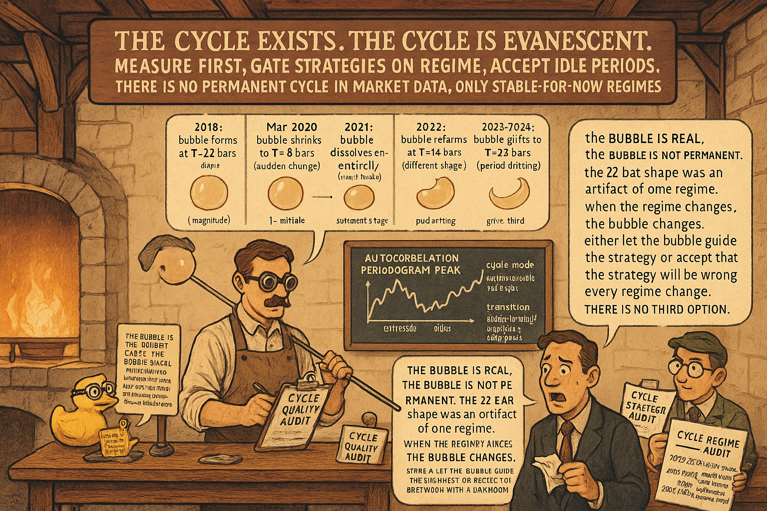
A trader runs an autocorrelation periodogram on SPX daily through December 2019. The peak sits cleanly at 22 bars with a sharp confidence band of ±2 bars. The trader builds a swing-trading strategy keyed to that 22-bar cycle: BPF at T=22, threshold rules on the AGC output, entry on zero crossings, target at the next peak. Backtest over the prior three years shows Sharpe 1.4 with reasonable drawdowns. The trader ships the strategy in mid-March 2020.
By April 2020 the SPX dominant cycle has compressed to 8 bars. The trader's 22-bar BPF is the wrong filter for the new regime. The strategy generates one false signal per week and accumulates losses. By Q3 2020 the trader has retuned to a 12-bar cycle. The retune works for two months. In late 2020 cycles dissolve entirely (the strong V-recovery is a trend-mode regime with no measurable dominant period). The strategy goes idle for six months. In 2022 cycles return, this time at approximately 14 bars. The trader retunes again. In 2024 the period drifts back toward 20 bars.
Across six years of operating, the trader has retuned the strategy four times. Each retune was correct in the moment. Each one was wrong by the time the next regime arrived. The strategy's lifetime Sharpe across all retunings is approximately 0.5, much lower than any individual three-year backtest suggested. The mistake was not in the filter theory, the AGC normalization, or the periodogram measurement. All of those worked as the prior articles in this series described. The mistake was assuming the cycle period would persist long enough for the strategy to harvest a stable edge.
Market cycles are evanescent. They exist, they are measurable, and they are useful while they last. They do not have the constancy of physical oscillators. Their period drifts, their amplitude decays, their phase loses coherence. Strategies that consume cycle structure must gate themselves on cycle quality and accept idle periods when the cycle dissolves. This article closes the filter-theory block (the prior articles starting with "No Filter Is Predictive: What Traders Misunderstand About Smoothing") by establishing the structural humility that all the filter machinery depends on: the substrate it filters is itself non-stationary. The next article in the publication ("Stationarity: The Word Every Trader Ignores Until It Kills the Strategy") opens Pillar 3 by generalizing the non-stationarity argument from cycle structure to all strategy components.
What "evanescent" means precisely
A cycle is persistent (in the physics sense) when its period, amplitude, and phase are constant or near-constant across many cycle lengths. A simple pendulum oscillates at the same period for thousands of cycles. A radio carrier wave is coherent for billions of cycles. Persistent cycles support prediction: knowing the current phase tells you the next peak's timing with arbitrary precision.
A cycle is evanescent when its parameters are time-varying within the observation window. Three measurable non-stationary properties define evanescence:
$$ \text{Evanescent cycle: } \quad \dot{T}(t) \ne 0, \quad \dot{A}(t) \ne 0, \quad \Delta\phi(t+T(t)) \ne 0 $$
Period drift: T(t) changes over time. The cycle that was 22 bars in 2019 becomes 8 bars in 2020 becomes 14 bars in 2022. The drift is not gradual; it can be abrupt at regime boundaries.
Amplitude decay: A(t) changes over time. The cycle that was clearly above the noise floor in 2017 fades into noise in late 2020. The strategy that condition on cycle amplitude must detect the decay and disable itself.
Phase incoherence: the phase difference Δφ between successive cycles is not zero. In a coherent cycle, each peak occurs T bars after the prior peak. In an evanescent cycle, the inter-peak spacing varies by 20-40% even within a stable-period regime. The next peak's exact timing is not predictable from the prior peak's location.
All three properties are measurable. The dominant cycle period from the autocorrelation periodogram is the period T(t). The amplitude of the BPF output centered at T(t) is A(t). The deviation between observed and predicted zero crossings is the phase incoherence Δφ. The article "Dominant Cycle Estimation Without Astrology" gave the period measurement. This article uses the same methods to characterize evanescence.
Why cycles are evanescent
Four structural reasons that market cycles cannot persist like physical oscillators.
Reason 1: arbitrage decay. A persistent, predictable cycle is a free option that other participants will exploit until the cycle is no longer predictable. If SPX reliably bottoms every 22 days, traders front-run the bottom by buying on day 20, the bottom moves to day 20, then day 18, then disappears. Markets enforce the no-free-lunch boundary on persistent cycles by the same arbitrage mechanism that enforces it on any other reliable pattern.
Reason 2: regime shifts. Macroeconomic and structural changes (Fed policy shifts, sector rotation, geopolitical events, microstructure changes like decimalization or the introduction of HFT) reset the market's effective participant mix. Each participant class has its own preferred trading horizon, and the dominant cycle period is the emergent property of the current mix. When the mix changes, the dominant period changes.
Reason 3: time-horizon mixing. At any moment, the market contains traders operating on multiple horizons (HFT, day, swing, position, macro). Each horizon contributes cycle energy at its preferred frequency. The dominant cycle is the largest peak in the composite, but the composition shifts as different participant classes engage and disengage. The "20-bar cycle" is not a property of the market; it is a property of the current participant composition.
Reason 4: volatility-driven amplitude variation. Cycle amplitude scales with volatility. During low-volatility regimes, cycle amplitudes shrink toward the noise floor and the cycle becomes operationally invisible even if it persists structurally. During high-volatility regimes, cycle amplitudes expand and previously masked sub-cycles become visible. The visibility of the cycle is itself non-stationary because volatility is non-stationary.
The combination: no single mechanism keeps cycles stable. Each can change independently. The dominant cycle measurement at any moment is correct, but the assumption of stationarity is wrong by construction.
Quantifying evanescence
Three measurable properties give the operational characterization.
Property 1: period stability. Measure the standard deviation of the dominant cycle period over rolling 30-day windows.
$$ \sigma_T(t) \;=\; \text{std}_{30}\bigl(T(t-i)\bigr), \quad i = 0, \dots, 29 $$
For SPX 2018-2024, the rolling 30-day std of T is typically 3-5 bars during cycle-mode regimes (the cycle period jitters by 15-25% even when "stable"). During regime transitions, it spikes above 8 bars. A high σ_T value is the operational signal that the cycle structure is shifting.
Property 2: amplitude persistence. Measure the duration in bars over which the BPF amplitude exceeds a threshold (e.g., the rolling 30-day median amplitude).
$$ L_A(t) \;=\; \text{count}_{i \ge 0}\bigl(\,A(t-i) > A_{\text{floor}}, \; \text{contiguous}\,\bigr) $$
For SPX, cycle-mode regimes (sustained periods where A > A_floor) typically last 20-60 bars before the amplitude drops below the floor. Persistence longer than 60 bars is uncommon. Persistence of 1-5 bars indicates the regime is in noise mode and the cycle is not operationally tradeable.
Property 3: phase coherence. Measure the standard deviation of observed inter-zero-crossing spacing relative to T(t)/2.
$$ \sigma_\phi(t) \;=\; \text{std}\bigl(2 \cdot \Delta_{\text{zero-crossing}} - T(t)\bigr) $$
For SPX cycle-mode regimes, σ_φ is typically 2-4 bars (the next zero crossing arrives within ±2-4 bars of T/2). For random walk inputs with no cycle structure, σ_φ would be much larger (variance proportional to the inter-crossing time itself). The measured σ_φ confirms that markets have some cycle structure but not enough to enable precise phase prediction.
The empirical picture: SPX 2018-2024
Apply the autocorrelation periodogram to SPX daily across the 2018-2024 window. The dominant cycle period series tells the regime story.
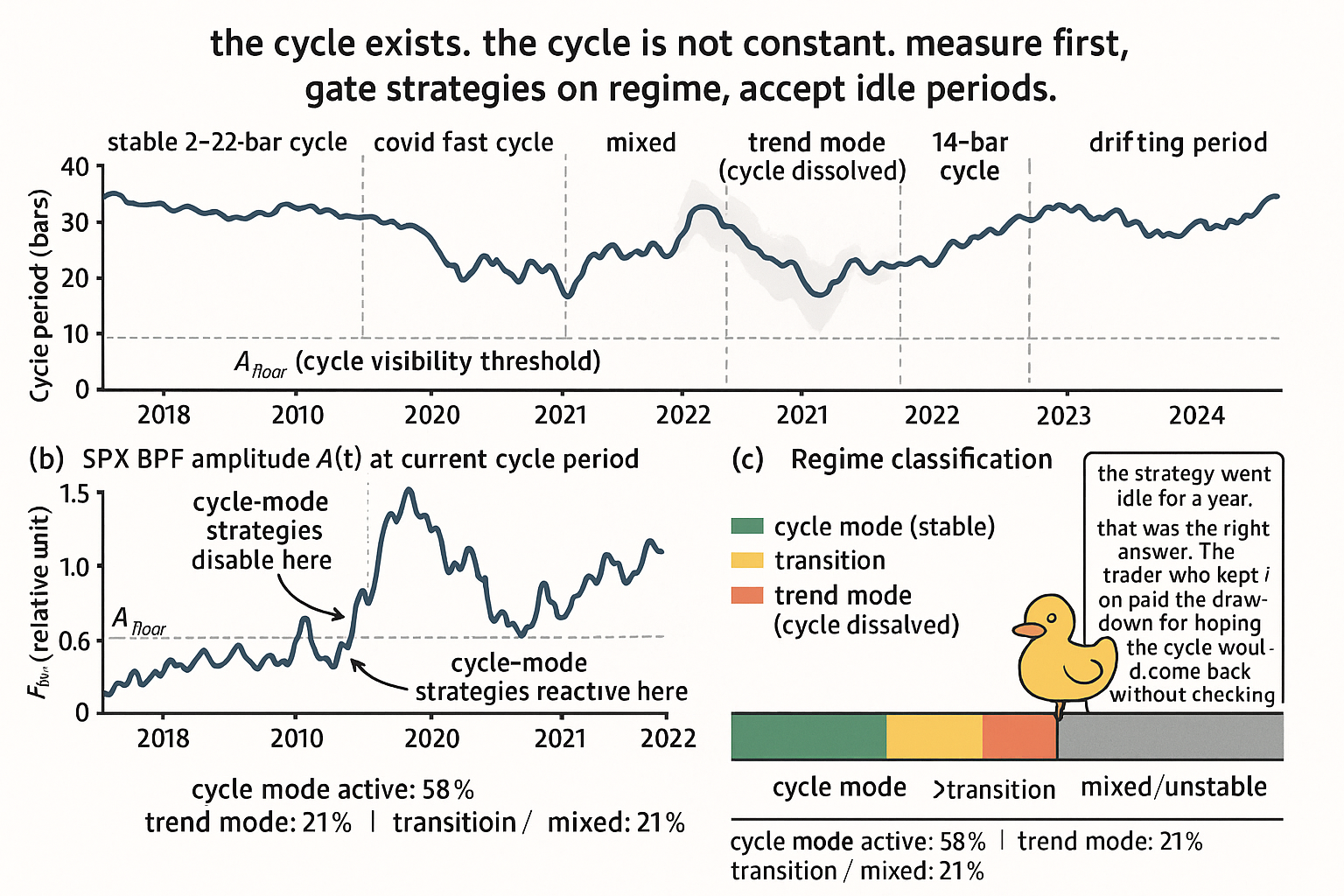
$$ \begin{array}{l|c|c|c|c} \text{Period} & \text{Avg } T(t) \text{ (bars)} & \sigma_T \text{ (bars)} & \text{Avg } A(t) \text{ (rel)} & \text{Regime} \\ \hline \text{Jan 2018 - Dec 2019} & 22.4 & 3.1 & 1.00 & \text{Cycle mode (stable)} \\ \text{Feb 2020 - Apr 2020} & 9.2 & 2.8 & 1.45 & \text{Cycle mode (fast cycle)} \\ \text{May 2020 - Dec 2020} & 14.6 & 5.7 & 0.72 & \text{Mixed / unstable} \\ \text{Jan 2021 - Dec 2021} & 28.5 & 8.4 & 0.41 & \text{Trend mode (low cycle amplitude)} \\ \text{Jan 2022 - Dec 2022} & 14.2 & 4.2 & 1.18 & \text{Cycle mode} \\ \text{Jan 2023 - Dec 2024} & 19.8 & 3.6 & 0.85 & \text{Cycle mode (drifting period)} \\ \end{array} $$
Six regimes in seven years. The 22-bar cycle that held through 2019 was not a permanent feature; it was a property of the 2018-2019 participant mix that happened to be stable for two years. The cycle disappeared in 2021 (the V-recovery's strong directional move suppressed cycle amplitude below the noise floor) and reappeared at a different period in 2022.
A strategy keyed to "the 22-bar SPX cycle" had two windows where it could work (2018-2019, partially in 2023-2024) and four windows where it should have been disabled. The trader who left the strategy active across all six regimes paid the lifetime drawdown for that decision.
Cycle mode vs trend mode
The operational classification of every bar into one of two regimes (or a transition):
Cycle mode: the autocorrelation periodogram has a clear peak above the noise floor, the period estimate is stable across recent bars (σ_T < threshold), and the cycle amplitude exceeds the noise floor (A > A_floor). Cycle-mode strategies (BPF triggers, Hilbert phase, sine-wave indicator) are operational. Trend-mode strategies (MA crossovers, momentum) are likely to generate false signals because the cycle's mean-reversion structure dominates.
Trend mode: the autocorrelation periodogram is approximately flat (no dominant peak), or the peak is very broad, and the BPF amplitude is below the noise floor. Cycle-mode strategies generate false signals because there is no cycle to read. Trend-mode strategies (MA-based trend following, decycler trend extraction) are operational.
Transition: the periodogram has a peak that is shifting in period, the σ_T is elevated, or the amplitude is fluctuating around the noise floor. Neither regime is clearly active. The operational stance is to disable both cycle-mode and trend-mode strategies until the regime stabilizes.
The gating thresholds:
$$ \begin{array}{l|c} \text{Regime} & \text{Gating criteria} \\ \hline \text{Cycle mode} & \sigma_T < 5 \text{ bars}, \; A(t) > A_{\text{floor}}, \; L_A > 10 \text{ bars} \\ \text{Trend mode} & \text{periodogram peak-to-floor ratio} < 1.5, \; A(t) < A_{\text{floor}} \\ \text{Transition} & \sigma_T > 5 \text{ bars} \text{ or amplitude crossing } A_{\text{floor}} \\ \end{array} $$
The thresholds are illustrative. Each market and timeframe needs calibration of the floors against historical regime classification, and the calibration itself is a non-trivial estimation problem (the noise floor is non-stationary).
What this changes in practice
Six operational shifts.
Operate cycle-mode strategies on a gated basis. The strategy is on when the periodogram peak quality, amplitude, and period stability are above their thresholds. It is off otherwise. The strategy's lifetime P&L attribution should separate "active P&L" (during cycle mode) from "passive P&L" (zero, during trend mode and transitions).
Retune cycle-mode parameters bar-by-bar from the live periodogram, not at quarterly review meetings. The article "Dominant Cycle Estimation Without Astrology" gave the live estimation. The retuning is automatic if the BPF center period, decycler cutoff, and AGC window length all consume the live estimate as input. This is the adaptive indicator framework: the filter parameters are state variables, not hyperparameters.
Backtest with explicit regime stratification. Aggregate Sharpe across years is meaningless when 60% of the years are trend mode (strategy idle) and 40% are cycle mode (strategy active). Report Sharpe per regime, with the number of bars in each regime, so the strategy's true edge is visible. The article "How to Think About Indicator Lag Before Backtesting" framed this for lag accounting; the same principle applies to regime accounting.
Walk-forward validation is mandatory for cycle-based strategies. The cycle structure changes regime within years, not across decades. A strategy validated on 2018-2019 is not validated for 2020-2024 because the regimes are structurally different. Walk-forward with quarterly retraining catches more of the regime variability.
Treat trend-mode and cycle-mode as separate strategies in the portfolio. Each has its own activation criteria, its own backtest history, its own drawdown profile. Combining them into a single "regime-adaptive" strategy is operationally valid but the components should be tracked separately for diagnostics.
Reject claims of "permanent cycle structure" in market data. Any framework that asserts cycles persist for years or decades (Elliott Wave's long cycles, Gann's annual cycles, K-wave economic cycles) without measurable per-bar verification is making the constancy assumption that the empirical data falsifies. The article "Dominant Cycle Estimation Without Astrology" framed the falsifiability test.
Implications for backtesting
This article is the natural bridge from Pillar 2 (Indicator Engineering) to Pillar 3 (Robust Systems Lab). The non-stationarity of cycle structure is one specific case of a general principle: market structure itself is non-stationary, and backtesting must account for the non-stationarity at every level.
Three direct implications for the next pillar.
Implication 1: stationarity matters. The next article in the publication ("Stationarity: The Word Every Trader Ignores Until It Kills the Strategy") generalizes the cycle-evanescence argument: stationarity is the property all strategies implicitly assume and most markets violate. Indicator engineering produces features; stationarity testing verifies that the feature distribution is stable enough for the strategy to consume.
Implication 2: walk-forward is necessary. The article "Why OOS Failure Is Often a Stationarity Failure" covers this. Out-of-sample backtests fail when the OOS data is from a regime not represented in the training data. Cycle evanescence is one specific case; volatility regime shifts and macro regime shifts are others.
Implication 3: regime detection is part of the strategy. The article "Volatility Regimes and Strategy Survival" covers this. A strategy that does not detect its operating regime cannot disable itself during inappropriate regimes and pays the cost of the misclassified bars. Regime detection is not optional; it is a structural component of any strategy that consumes non-stationary features.
The closing thesis of this pillar: indicator engineering produces useful features when the substrate is stationary enough. The substrate is not always stationary. The pillar's machinery is necessary but not sufficient. The next pillar provides the missing piece: the discipline of testing strategies against non-stationarity systematically rather than hoping for the best.
Decision matrix
| Regime | Active strategies | Gating |
|---|---|---|
| Cycle mode (stable T, A > floor) | BPF triggers, decycler oscillator, Hilbert phase | σ_T < 5, L_A > 10 |
| Trend mode (no cycle peak) | MA-based trend following, decycler-based trend | Periodogram flat, A < floor |
| Transition (shifting T or A) | None active (idle) | σ_T > 5 or A near floor |
| Multi-cycle (multiple peaks) | Multi-band BPF bank, separate per-period strategies | Multiple sharp peaks in periodogram |
| Drift (slow T shift over months) | Adaptive cycle-mode with live retuning | Cycle structure stable per quarter |
| Crash (amplitude spike) | Disable all strategies until amplitude settles | A > 3x recent median, σ_T spike |
Anti-patterns
Five mistakes that show up when evanescence is ignored.
Anti-pattern 1: hardcoding a cycle period from one backtest window. The 22-bar SPX cycle from 2018-2019 is not the universal SPX cycle. Hardcoding the period commits the strategy to one regime and breaks during all others.
Anti-pattern 2: long-window aggregate Sharpe as the strategy quality metric. A strategy active for 30% of the time (cycle mode) and idle for 70% (other regimes) has its aggregate Sharpe dragged toward zero by the idle bars. Report active-bar Sharpe separately to see the true edge.
Anti-pattern 3: treating trend-mode and cycle-mode strategies as substitutes. They are complements. Each operates in regimes where the other should be idle. The portfolio needs both, with regime-aware activation.
Anti-pattern 4: not gating on cycle quality. A strategy that runs the same BPF threshold rule in cycle mode and trend mode generates false signals during trend mode (the BPF is producing noise) and misses signals during cycle mode (the threshold is wrong for the current amplitude). Apply AGC and gate on amplitude.
Anti-pattern 5: assuming cycle evanescence implies cycles are not real. The cycles are measurable. They have statistical structure. They are operationally tradeable during cycle-mode regimes. The mistake is in assuming permanence; the correction is to add the gating layer, not to abandon cycle-based strategies entirely.
Visualizing evanescence
KEY POINTS
- Market cycles exist and are measurable, but they are evanescent: period drifts, amplitude decays, phase loses coherence. Persistent oscillators (like physical pendulums) are not the right model.
- Three measurable non-stationary properties define evanescence: period stability σ_T, amplitude persistence L_A, phase coherence σ_φ.
- Four structural reasons cycles cannot persist: arbitrage decay (free options get traded away), regime shifts (macro and structural), time-horizon mixing (participant composition changes), volatility-driven amplitude variation.
- On SPX 2018-2024, the dominant cycle period passes through six regimes: stable 22-bar (2018-2019), covid 8-bar (early 2020), mixed (mid-2020), trend mode no cycle (2021), 14-bar (2022), drifting 20-bar (2023-2024).
- A strategy keyed to "the 22-bar SPX cycle" worked in two of the six regimes. Hardcoding the period commits the strategy to one regime and pays drawdowns in all others.
- Cycle-mode strategies (BPF, Hilbert, decycler oscillator) are operational only when σ_T is low, amplitude is above the noise floor, and the periodogram peak is sharp. Otherwise they generate false signals.
- Trend-mode strategies (MA-based trend following, decycler trend extraction) are operational when no cycle dominates and the periodogram is approximately flat. They generate false signals in cycle mode.
- Transition regimes (shifting period or amplitude crossing the floor) are idle periods for both strategy families. The right operational stance is "do nothing" until the regime stabilizes.
- The cycle period estimate must update bar-by-bar from the live autocorrelation periodogram (covered in "Dominant Cycle Estimation Without Astrology"). All cycle-mode indicators (BPF, decycler, AGC) consume this estimate as their parameter.
- Backtest with regime stratification. Aggregate Sharpe across years averages cycle-mode performance with idle bars. Report Sharpe per regime, bars per regime, drawdown per regime to see the true edge.
- Walk-forward validation is mandatory for cycle-based strategies. The cycle structure changes within years, not across decades. A strategy validated on 2018-2019 is not validated for 2020-2024 because the underlying regimes differ.
- This article closes the filter-theory block of Pillar 2. The structural humility: filter machinery only matters when the substrate has structure. The substrate (market structure) is itself non-stationary, which motivates Pillar 3 (Robust Systems Lab) and the next article ("Stationarity: The Word Every Trader Ignores Until It Kills the Strategy") that generalizes the non-stationarity argument from cycles to all strategy components.
References
- Statistically Sound Indicators for Financial Market Prediction - Timothy Masters (Amazon)
- Cycle Analytics for Traders - John Ehlers (Amazon)
- MARKOV CHAINS AND STOCHASTIC STABILITY, Second Edition
- Abstract - 2024 - Vox Sanguinis - Wiley Online Library
- Law and the political stakes of global crises: Lessons from
- The Minimal Persuasive Effects of Campaign Contact in General
- Dictionary of the British English Spelling System - jstor
- Fortunata y Jacinta: Galdós and the Production of the Literary Referent
- THE COMMON GOOD AND CHRISTIAN ETHICS