2.27 How to Think About Indicator Lag Before Backtesting
Every linear indicator has known lag. Sum cascades, compare to time-to-half-move. EMA+RSI on 5-bar mean reversion: 17-bar lag, structurally broken. Audit lag before backtesting, not after deployment.
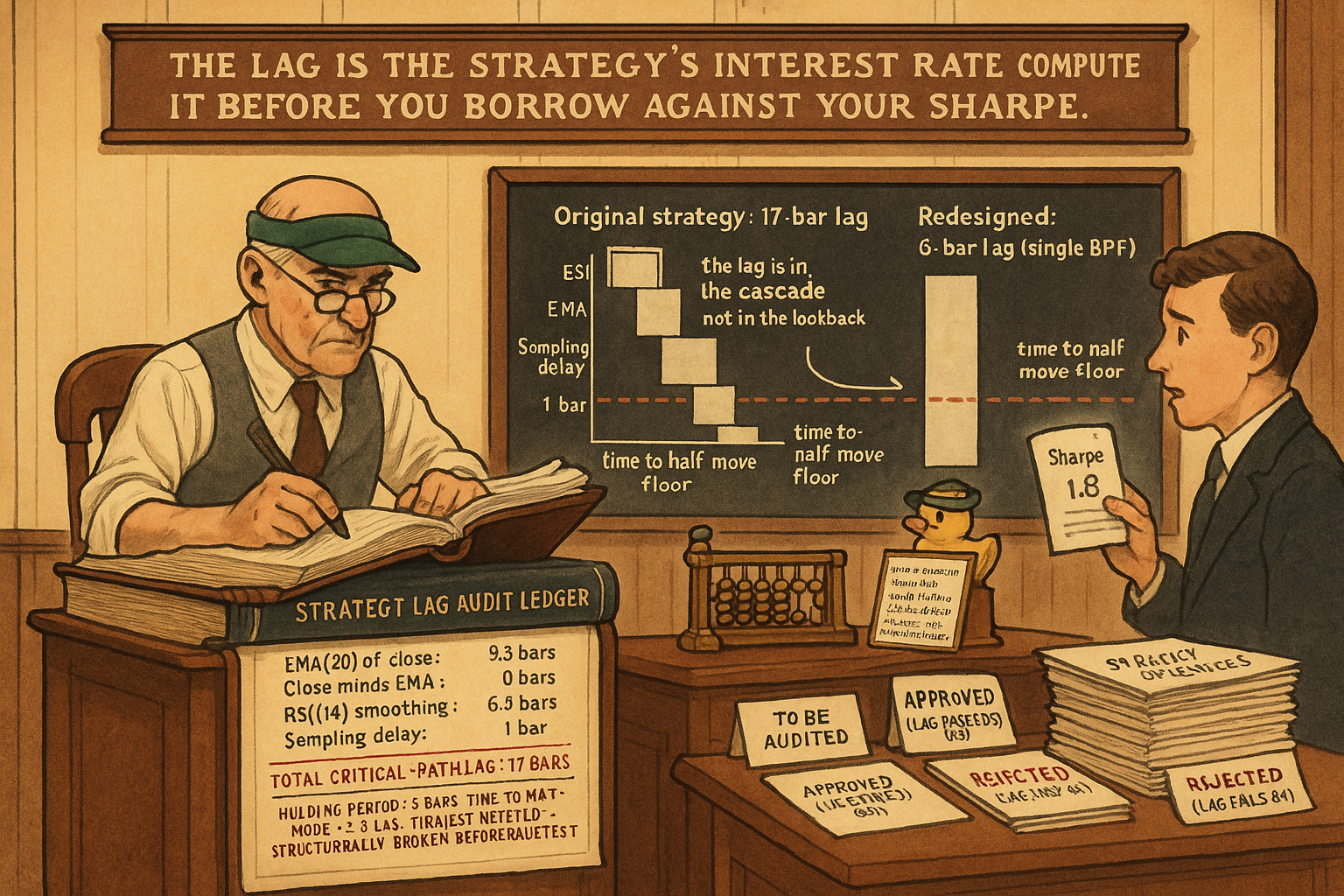
A trader designs a mean-reversion strategy on SPX daily. The construction: smooth the close with EMA(20), compute close-minus-EMA, feed into RSI(14), trigger long entries when RSI dips below 30. The trader runs the backtest, sees Sharpe 1.8 over 15 years, and ships to paper trading. Two months later the live results show Sharpe 0.4 with negative skew. The trader blames "regime change" and shelves the strategy.
The strategy did not fail because the regime changed. It failed because the backtest ran without a lag audit. The EMA(20) introduces 9.5 bars of group delay. The RSI(14)'s internal EMA introduces another 6.5 bars of cascade lag at the cycle frequencies the strategy targets. The combined critical-path lag is approximately 16 bars. The strategy's target holding period is 5 bars (mean-reversion to the EMA, typically completing in less than a week). The lag is more than three times the holding period. Every signal arrives so late that the mean reversion has already happened by the time the entry triggers.
The backtest showed Sharpe 1.8 because the backtest engine, like every backtest engine, runs the signal computation on time-indexed data without distinguishing between "what the trader sees now" and "what the data eventually showed at this timestamp." The 16-bar lag was absorbed into the backtest as look-ahead masquerading as smoothing. Live trading exposes the lag because the trader cannot wait for the smoothed value to stabilize before placing the trade.
The article "The Hidden Cost of Every Moving Average: Lag" established the structural lag of common smoothers. The article "Why Moving Averages Can Lie at Turning Points" showed the lag's operational cost at structural inflection points. The article "The Frequency Response of Trading Indicators" gave the universal framework for reading any linear indicator's response. This article gives the pre-backtest planning discipline: how to compute the lag budget of a proposed strategy, compare it to the holding period and the expected move time, and make the go-or-no-go decision before the first backtest run.
The next article in this series ("Why Median Filters Are Useful for Volume and Outliers") covers a class of nonlinear filters whose lag properties differ from linear filters in operationally useful ways.
What lag actually means
Two formal definitions of lag, both derived from the filter's transfer function H(z). Either can be the right answer depending on what part of the signal the strategy uses.
Group delay: the delay applied to the envelope of a wavetrain at frequency ω. Derived from the negative derivative of the phase response:
$$ \tau_{\text{group}}(\omega) \;=\; -\frac{d \arg(H(e^{j\omega}))}{d \omega} $$
Group delay matters when the strategy reads the indicator's level or trend (slope). The level at time t reflects the data from t minus τ_group bars ago.
Phase delay: the delay applied to a single sinusoid at frequency ω. The ratio of the phase to the frequency:
$$ \tau_{\text{phase}}(\omega) \;=\; -\frac{\arg(H(e^{j\omega}))}{\omega} $$
Phase delay matters when the strategy reads the indicator's cycle position (zero crossing, peak, trough). The cycle at time t crosses zero τ_phase bars later than the underlying data does.
For a symmetric FIR filter (SMA, Hann window, Blackman window) the two delays are equal and constant across all frequencies. For an IIR filter (EMA, recursive HPF/LPF, BPF) the two delays are frequency-dependent and not equal to each other.
The operational shortcut: for any linear indicator, compute the lag at the dominant frequency of the cycle being read. That is the lag the strategy pays.
Lag formulas for the standard toolkit
Lag in bars at the cycle frequency for which each filter is designed.
$$ \begin{array}{l|c|c} \text{Filter} & \text{Lag formula} & \text{Lag (bars) at default lookback} \\ \hline \text{SMA}(N) & (N-1)/2 & 9.5 \text{ for } N{=}20, \; 24.5 \text{ for } N{=}50 \\ \text{EMA}(\alpha) & (1-\alpha)/(2\alpha) \approx (N-1)/2 & 9.5 \text{ for } N{=}20, \; 24.5 \text{ for } N{=}50 \\ \text{WMA}(N) & (N-1)/3 & 6.3 \text{ for } N{=}20 \\ \text{1-pole LPF (cutoff T)} & \approx T/(2\pi) & 3.2 \text{ for } T{=}20 \\ \text{2-pole LPF (cutoff T)} & \approx T/\pi & 6.4 \text{ for } T{=}20 \\ \text{Super-smoother (T)} & \approx T/2 & 10 \text{ for } T{=}20 \\ \text{1-pole HPF (cutoff T)} & \approx T/(2\pi) & 3.2 \text{ for } T{=}20 \\ \text{2-pole HPF (cutoff T)} & \approx T/\pi & 6.4 \text{ for } T{=}20 \\ \text{BPF (center T, } \delta{=}0.3) & \approx T/3 \text{ to } T/4 & 5.0 \text{ to } 6.7 \text{ for } T{=}20 \\ \text{Decycler (HPF cutoff T)} & \approx T/(2\pi) & 14.5 \text{ for } T{=}30 \\ \text{Differencer } x_t - x_{t-1} & 0.5 & 0.5 \\ \text{N-bar momentum } x_t - x_{t-N} & N/2 & 10 \text{ for } N{=}20 \\ \end{array} $$
Twelve formulas. The lag of every linear operation in the strategy is computable from this table in seconds.
The numbers reveal the structural tradeoffs covered in prior articles. Same-cutoff comparison: a 1-pole LPF has roughly half the lag of a super-smoother but lets through about ten times more cycle leakage. The BPF has comparable lag to a 2-pole LPF but operates on a much narrower frequency band.
The lag budget
The lag budget of a strategy is the sum of the lags of the linear operations along the critical signal path, plus any sampling and execution delays.
Critical signal path: the longest sequence of linear operations from input data to trade decision. Branching computations (e.g., two indicators evaluated in parallel and combined) take the maximum of the two branch lags, not the sum.
Cascade rule: when one filter's output feeds another's input (cascade), the lags add. Two EMA(20)s in series produce a 2-pole-like response with combined lag 9.5 + 9.5 = 19 bars at the dominant frequency.
Parallel rule: when two filters operate on the same input and their outputs are combined linearly (sum, difference), the resulting filter's lag is the lag of the slower branch in the band where it dominates. For MACD = EMA(12) − EMA(26), the lag is approximately the EMA(26) lag (12.5 bars) at the cycle band where MACD peaks.
Nonlinearity rule: nonlinear operations (gain/loss separation in RSI, range normalization in Stochastic, max/min over rolling window) do not change the underlying linear filter's lag. They shape the output distribution but the cycle-band reading still happens at the linear filter's lag.
Sampling delay: a strategy that decides on the close of bar t and executes on the open of bar t+1 carries a 0.5 to 1 bar sampling delay. This is structural for any close-of-bar strategy.
Filter warmup: the first N bars of any filter's output are not at the filter's steady-state response. The warmup adds lag during the first N bars of operation. After warmup, the lag is at the table values.
The full budget:
$$ \tau_{\text{budget}} \;=\; \sum_{\text{operations on critical path}} \tau_{\text{filter}} \;+\; \tau_{\text{sampling}} \;+\; \tau_{\text{warmup correction (if applicable)}} $$
For the opening example (EMA(20) → close-minus-EMA → RSI(14) → trigger): - EMA(20): 9.5 bars - Close minus EMA: 0 bars (subtraction has no lag) - RSI(14)'s internal EMA on gains and losses: 6.5 bars - Sampling delay: 1 bar - Total: 17 bars
Critical-path lag for the strategy: 17 bars. Holding period for the strategy: 5 bars. The lag is 3.4 times the holding period. The strategy has no operational room for its own decision latency.
The four costs of lag
Lag is not a single number on a P&L line. It produces four distinct costs that each show up at different stages of the strategy lifecycle.
Cost 1: missed move. By the time the signal fires, part of the move has already happened. For a 5% move that takes 10 bars to develop, a 5-bar lag captures about 50% of the move. A 15-bar lag captures roughly zero (the move is over).
Cost 2: stale state. The indicator level read at time t reflects the data from t minus τ bars ago. Strategies that condition on level (close above EMA, RSI below 30) are conditioning on a state that no longer exists. The decision is made against past truth.
Cost 3: false signals. Lag makes filters slow to respond to true regime changes but fast to respond to phantom regime changes (transient noise that the slow filter integrates as a real shift). The article "Why the SMA Is Often a Terrible Smoother" detailed the sidelobe-induced false signal problem.
Cost 4: P&L attribution corruption. The backtest's reported edge mixes (a) true forecasting alpha and (b) lag-absorbed look-ahead. The two cannot be separated without explicit lag accounting. Strategies that look strong in backtest and fail in live are typically those where the lag-absorbed component was larger than the true alpha.
Pre-backtest checklist
Four questions, answered in order, before any backtest runs.
Q1: What is the lag budget? Sum the lags of every linear operation on the critical path. Add sampling delay and any warmup correction. Express in bars.
Q2: What is the holding period? For a strategy with explicit holding period (exit after N bars), this is N. For a strategy with dynamic exit (target or stop), use the median historical hold across similar strategies as the estimate. If no estimate exists, the strategy specification is incomplete.
Q3: What is the time-to-half-move? For the typical winning trade, how many bars does it take for half the move to develop? This is the bar count after which a late signal stops being useful. For mean-reversion to an MA, time-to-half-move is roughly the band's typical reversion time, often 2-5 bars. For trend-following moves, time-to-half-move is roughly half the trend's typical duration, often 20-50 bars.
Q4: Is the lag budget less than half the time-to-half-move? If yes, the strategy has room. The lag is small enough that the signal arrives while the move is still unfolding. If no, the strategy is structurally late and will lose the bulk of every move to the lag.
A failed Q4 means the strategy needs redesign before backtesting. Either reduce the lag (replace cascaded filters with single-stage filters, switch from MA-based detection to cycle-mode detection) or accept a longer holding period that matches the lag budget.
Worked example: mean-reversion strategy redesign
The opening example, audited and redesigned.
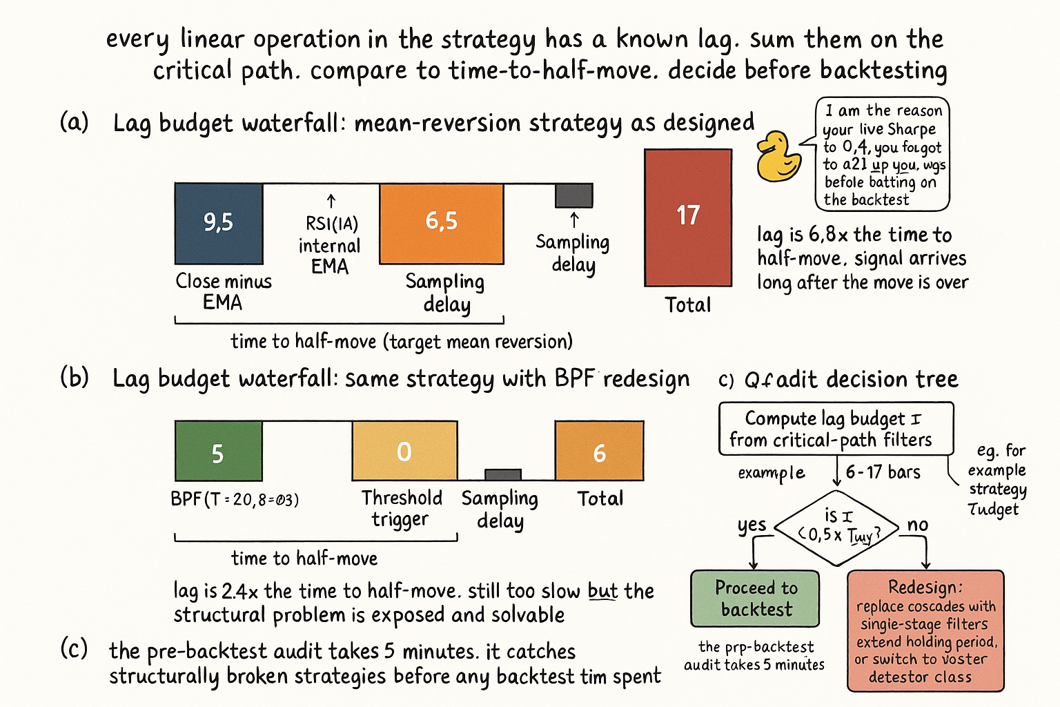
Original construction:
$$ \begin{array}{l|c} \text{Operation} & \text{Lag (bars)} \\ \hline \text{EMA(20) of close} & 9.5 \\ \text{Close minus EMA} & 0 \\ \text{RSI(14) on the deviation} & 6.5 \\ \text{Sampling delay (close-to-next-open)} & 1.0 \\ \hline \text{Critical-path lag} & 17.0 \\ \end{array} $$
Holding period: 5 bars. Time-to-half-move (for mean reversion to the EMA): 2.5 bars. Lag budget: 17 bars. The lag is 6.8 times the time-to-half-move. Q4 fails catastrophically. The strategy is structurally broken.
Redesigned construction using a single BPF for the same cycle band:
$$ \begin{array}{l|c} \text{Operation} & \text{Lag (bars)} \\ \hline \text{BPF(T=20, } \delta{=}0.3\text{) of close} & 5.0 \\ \text{Threshold trigger on BPF output} & 0 \\ \text{Sampling delay (close-to-next-open)} & 1.0 \\ \hline \text{Critical-path lag} & 6.0 \\ \end{array} $$
Critical-path lag: 6 bars. Holding period: 5 bars. Time-to-half-move: 2.5 bars. The lag is 2.4 times the time-to-half-move. Q4 still fails, but less severely.
Final redesign: extend the holding period to match the lag, or use a faster cycle-mode detector.
Option A: extend the holding period to 10 bars (target reversion to 20-bar BPF's full half-cycle). Time-to-half-move becomes 5 bars. Lag budget (6) is now 1.2 times the time-to-half-move. Q4 still marginal.
Option B: switch to a faster cycle detector, the autocorr reversal indicator covered in the article "Why Markets Are Not Random: The Autocorrelation Story", with lag of 2-4 bars. Lag budget drops to 3-5 bars. Q4 passes for the original 5-bar holding period.
The pre-backtest audit takes 5 minutes and saves weeks of backtesting work on a strategy that was structurally broken before the first run.
Hidden lag sources
Three sources of lag that do not appear in the transfer function but contribute to the operational lag budget.
Hidden source 1: lookback bias. Many backtest engines compute the signal at bar t using close[t], then assume the trade fills at close[t] or open[t+1]. If the indicator computation requires close[t] to produce the bar-t signal, the trade cannot fill until open[t+1] at earliest. The strategy specification must distinguish between "signal computed at close of t" and "trade filled at open of t+1." The 1-bar sampling delay is the minimum; any close-of-bar strategy has at least this lag.
Hidden source 2: filter initialization. The first N bars of any IIR filter's output are not at the steady-state response. For an EMA(50), the first 50-100 bars are warming up. For a BPF, the first 4T bars are warming up. Backtests that start at bar 1 carry warmup artifacts that look like signal. The fix: discard the warmup bars from the backtest results and start measurement only after the filter has stabilized.
Hidden source 3: data revision. For intraday data, the close of the bar is sometimes revised after the bar closes (exchange corrections, late prints). Strategies that depend on the close of the most recent bar for the current bar's signal cannot trade until after the revision window closes. This adds operational lag that is invisible in backtest data because the backtest sees only the final values.
Each hidden source adds 1 to 5 bars of operational lag that the transfer-function calculation misses. Pre-backtest budgeting should include explicit estimates of each.
What this changes in practice
Five operational shifts.
Compute the lag budget before any backtest. The budget is a 5-minute calculation. It catches structurally broken strategies before any computation time is spent.
Report strategy performance with the lag explicit. The line "Sharpe 1.8 (16-bar lag budget, 5-bar holding period)" is honest. The line "Sharpe 1.8" is misleading because the reader cannot tell whether the edge survives the lag.
Choose holding period and lag budget together. A 5-bar holding period mandates a sub-2-bar lag budget. A 50-bar holding period tolerates 10-15 bars of lag. The two parameters are jointly chosen, not separately optimized.
Cap indicator cascades. If the lag budget is 5 bars, the strategy cannot use any cascade longer than 5 bars / typical_filter_lag operations. Cascading three EMAs (28-bar combined lag) on a 5-bar holding period is mechanically broken.
Reject strategies that fail Q4 at design time. A strategy with 17-bar lag on a 5-bar holding period is not "interesting to backtest." It is structurally broken. Spend the backtest time on strategies that pass the lag audit.
Decision matrix
| Holding period | Max lag budget | Allowed constructions |
|---|---|---|
| 1-3 bars (intraday, scalp) | 1-2 bars | Differencer, 1-bar momentum, no smoothing |
| 5-10 bars (short swing) | 3-5 bars | BPF at cycle, fast EMA, decycler |
| 20-50 bars (medium swing) | 10-15 bars | EMA(20-30), super-smoother, decycler |
| 50-200 bars (position) | 25-50 bars | EMA(50-100), slow super-smoother |
| 200+ bars (regime) | 50-100 bars | Long-term decycler, multi-pole LPF |
| Cycle-mode (BPF zero cross) | T/4 to T/3 | BPF at cycle period |
| Turning point (cycle-mode) | 2-5 bars | Autocorr reversal, Hilbert phase |
| Mean reversion (1-3 bar) | 1-2 bars | Differencer-based trigger |
Anti-patterns
Five mistakes that show up in strategy backtests.
Anti-pattern 1: optimizing lookbacks against backtest P&L without lag accounting. The optimization will find lookbacks where the lag-absorbed look-ahead is largest. The resulting strategy fails in live.
Anti-pattern 2: cascading three or four indicators without summing the lags. A common construction: "smooth with EMA, normalize with rolling std, smooth again, threshold." Each step adds 5-10 bars. The composite lag is 20-30 bars and the strategy targets 5-bar moves. Mechanically impossible.
Anti-pattern 3: treating "EMA(50) is still up" as a present-tense reading. The EMA's value at time t reflects the trend 25 bars ago. A strategy that conditions on this for a 5-bar trade is using stale state.
Anti-pattern 4: assuming "we'll fix it in optimization" works for lag. Lag is structural, not a hyperparameter. Optimization can only move along the lag-vs-noise Pareto frontier; it cannot escape the frontier.
Anti-pattern 5: backtesting filter-based strategies with no warmup discard. The first N bars of any IIR filter are not at steady state. Including those bars in the backtest's Sharpe calculation inflates the result by the warmup artifact.
Visualizing the lag budget
KEY POINTS
- Every linear indicator has a known lag derived from its transfer function. The lag is computable from a small table for every filter in the standard toolkit.
- Group delay is the lag of the indicator's level and slope. Phase delay is the lag of the indicator's cycle position (zero crossings). Use whichever matches the strategy's signal source.
- The lag budget is the sum of the lags of every linear operation on the critical signal path, plus sampling delay and any warmup correction.
- Cascade rule: lags add. Two EMA(20)s in series carry 19 bars of lag. Parallel rule: lags take the maximum of the dominant branch. Nonlinearity rule: nonlinear shaping does not change the underlying linear filter's lag.
- Pre-backtest checklist: lag budget, holding period, time-to-half-move, Q4 (lag less than half the time-to-half-move?). A failed Q4 means the strategy is structurally broken and must be redesigned before any backtest runs.
- Common construction failure: EMA + RSI cascade for mean-reversion. Critical-path lag 17 bars, holding period 5 bars, lag-to-holding ratio 3.4. The lag absorbs the move before the signal fires.
- Redesign with a single BPF at the same cycle band cuts lag from 17 to 6 bars. Further redesign with autocorr reversal or Hilbert phase brings it under 4 bars and passes Q4.
- Hidden lag sources: lookback bias (close-of-bar strategies have at least 1-bar sampling delay), filter initialization (IIR warmup), data revision (intraday close revisions).
- Backtests that report Sharpe without disclosing lag are misleading. Sharpe and lag are jointly meaningful. Report both.
- Holding period and lag budget are jointly chosen. A 5-bar holding period mandates a sub-2-bar lag budget. A 50-bar holding period tolerates 10-15 bars. The two parameters are not separately optimizable.
- Lag is not a hyperparameter. Optimization moves along the lag-vs-noise Pareto frontier but cannot escape it. The escape comes from changing construction class, not from tuning.
- Anti-pattern: "we'll fix it in backtest optimization." Lag failures show up in backtest as look-ahead-absorbed Sharpe that disappears in live. The fix is structural redesign, not tuning.
References
- Statistically Sound Indicators for Financial Market Prediction - Timothy Masters (Amazon)
- Cycle Analytics for Traders - John Ehlers (Amazon)
- Lasse H
- DeltaLag: Learning Dynamic Lead-Lag Patterns in Financial Markets
- Linear Cointegration of Nonlinear Time Series with an Application to
- On the Intersection of Signal Processing and Machine Learning - arXiv
- arXiv:1907.09452v1 [q-fin.ST] 13 Jul 2019