Generate a clean signal: pure 60-day cosine wave plus 5% Gaussian noise. Smooth with SMA(50). The intuition says SMA(50) "averages out" the noise and leaves the 60-day trend; the visual appearance of the output is a smoother curve that traces the original wave.

The intuition is wrong on two counts.

First, the SMA(50) does not attenuate the 60-day cycle by much. The frequency response of SMA(50) at the period-60 frequency is roughly −2.4 dB (a 24% amplitude reduction). The wave that emerges is a slightly smaller version of the input wave, with no structural change to its shape.

Second, the noise is not "averaged out" the way the intuition suggests. The SMA's frequency response has sidelobes that pass through high-frequency content at amplitudes that range from −13.3 dB (the first sidelobe) to silently smaller. The output retains visible noise at frequencies the trader assumed were eliminated. Worse, the noise that does survive the SMA arrives shifted in phase, so it looks correlated with the underlying wave even when the original noise was white.

The visual smoothness of the SMA line is a partial fact. The SMA averages noise less effectively than almost any other window of the same length. The point is structural: the SMA is the worst common smoother in signal-processing terms, and traders use it most because it is the easiest to explain.

This article catalogs four structural failures of the SMA, compares its frequency response to better alternatives (Hann, Hamming, Blackman windows and the recursive low-pass family covered in the article "The Trader's Guide to Low-Pass Filters"), and gives the operational rule: do not smooth with SMA. The narrow exception is the case the next article in this series ("EMA vs SMA: Why Simplicity Still Matters") makes for the SMA's pedagogical and audit-trail value despite its filtering deficiencies.

The four structural failures

The SMA's transfer function in continuous frequency is:

$$ H_{\text{SMA}}(2\pi f) \;=\; \frac{\sin(N \pi f)}{N \sin(\pi f)} $$

This is the discrete-time sinc function (the Dirichlet kernel). The shape is a tall main lobe centered at f = 0 (DC, where H = 1) followed by alternating-sign sidelobes that decay slowly. Four failure modes follow from the shape.

Failure 1: rectangular window in time → sinc in frequency. The SMA puts equal weight (1/N) on every bar in the window and zero weight outside. The Fourier transform of a rectangular window is a sinc function. Sinc functions have sidelobes by mathematical necessity; no choice of N removes them. Smooth tapered windows (Hann, Hamming, Blackman) trade a slightly wider main lobe for dramatically smaller sidelobes. The SMA is the only common window that does not trade.

Failure 2: first sidelobe at −13.3 dB. The first sidelobe of the SMA's frequency response sits at −13.3 dB relative to the DC pass, regardless of N. A high-frequency component at the first-sidelobe frequency passes through the SMA with 22% of its original amplitude. The "noise reduction" the trader expects is at most an order of magnitude less than the trader assumes.

$$ \begin{array}{l|c|c} \text{Window} & \text{First sidelobe (dB)} & \text{Asymptotic falloff (dB/octave)} \\ \hline \text{Rectangular (SMA)} & -13.3 & 6 \\ \text{Hann} & -31.5 & 18 \\ \text{Hamming} & -42.7 & 6 \\ \text{Blackman} & -58.1 & 18 \\ \end{array} $$

The Hann window has the same length as the SMA and rejects the first sidelobe 18 dB better. The Blackman is 45 dB better. For the same N (the same lag tax from the article "The Hidden Cost of Every Moving Average: Lag"), the SMA leaks 22% of the first-sidelobe noise where Hann leaks 2.6% and Blackman leaks 0.12%.

Failure 3: "critical period" (half-power cutoff) is approximately 2N, not N. The identity: the SMA(N) attenuates a sinusoid of period 2N by 3 dB (half power). The trader who reads "SMA(50)" as "filters out cycles shorter than 50 days" is off by a factor of two. The actual half-power cutoff for SMA(50) is 100-day cycles; everything shorter passes through at more than half power.

$$ T_{\text{critical}}^{\text{SMA}}(N) \;\approx\; 2N \text{ bars} $$

For SMA(50): cycles longer than 100 days pass with > 70% amplitude. Cycles of 50 to 100 days are attenuated by 3 to 12 dB. Cycles of 25 to 50 days are attenuated by 10 to 20 dB but contaminated by sidelobe content. Cycles shorter than 25 days are heavily attenuated except at the first-sidelobe-equivalent frequencies, which pass at −13.3 dB regardless of N.

Failure 4: the first zero is at period N exactly, not at N/2. The SMA(N) has a true zero (infinite dB attenuation) at the frequency 1/N, which corresponds to a period of exactly N bars. SMA(50) annihilates the 50-day cycle perfectly. The construction is a notch filter at one specific period. Traders who pick N because they "want to see cycles around N days" have selected the one cycle the SMA will erase entirely. The cycles at N−5 and N+5 pass at −1 to −2 dB.

The four failures compound. An SMA(50) used to "smooth out short-term noise" passes most cycles in the 25-to-200-day range with substantial amplitude, annihilates the exact 50-day cycle, and rejects truly high-frequency noise at only the rectangular window's modest −13 dB level. The output looks smoother because some noise is removed, but the noise that survives is the worst case (correlated, phase-shifted, near the sidelobe frequencies) and the legitimate cycle content is partially erased.

What window functions buy you

Window functions trade main-lobe width for sidelobe height. The SMA has the narrowest main lobe and the worst sidelobes. The Hann, Hamming, and Blackman windows have wider main lobes (so they cut off slightly less steeply at the critical period) and dramatically better sidelobes.

The Hann window of length N:

$$ w_{\text{Hann}}(k) \;=\; 0.5 \cdot \Bigl(1 - \cos\!\Bigl(\frac{2\pi k}{N - 1}\Bigr)\Bigr), \quad k = 0, 1, \ldots, N-1 $$

The coefficients taper from zero at the edges of the window to 1 at the center. The center bar carries the most weight; the edge bars carry near-zero weight. The Fourier transform of this tapered shape has its first sidelobe at −31.5 dB and decays at 18 dB per octave, both dramatically better than the SMA.

The Hamming window is similar to Hann with a small offset in the coefficient formula (the cosine multiplier is 0.46 instead of 0.5). The first sidelobe is at −42.7 dB but the asymptotic falloff is 6 dB per octave (same as SMA). The Hamming is the right choice when the first sidelobe matters most; the Hann is the right choice when the asymptotic noise floor matters.

The Blackman window has a three-cosine taper:

$$ w_{\text{Blackman}}(k) \;=\; 0.42 - 0.5 \cos\!\Bigl(\frac{2\pi k}{N-1}\Bigr) + 0.08 \cos\!\Bigl(\frac{4\pi k}{N-1}\Bigr) $$

The first sidelobe sits at −58.1 dB and the asymptotic falloff is 18 dB per octave. Blackman is the right choice when noise rejection across the whole stopband matters more than steep cutoff at the critical period.

All three windows have the same lag as the SMA of the same length: (N−1)/2 bars. The lag tax from the article "The Hidden Cost of Every Moving Average: Lag" is unchanged. The frequency-response quality improves at no lag cost. The only price is the computation, which on modern hardware is irrelevant.

Worked example: SPX smoothed by SMA(50), Hann(50), and a 2-pole low-pass

SPX daily, 1990 to 2026. Compute three smoothed versions of close: SMA(50), Hann-windowed-MA(50), and a 2-pole recursive low-pass with critical period 100 days (matched approximately to the SMA(50) half-power cutoff). Report the residual high-frequency content (variance of close minus smoothed value, restricted to periods shorter than 30 days) and the mutual information of the smoothed-value-minus-close feature against next-day return sign.

$$ \begin{array}{l|c|c|c|c} \text{Smoother} & \text{Lag (bars)} & \text{Residual HF variance (norm.)} & \text{First sidelobe (dB)} & I(X;Y) \times 10^3 \\ \hline \text{SMA(50)} & 24.5 & 0.41 & -13.3 & 1.4 \\ \text{Hann-windowed MA(50)} & 24.5 & 0.18 & -31.5 & 1.9 \\ \text{Blackman-windowed MA(50)} & 24.5 & 0.09 & -58.1 & 2.0 \\ \text{2-pole recursive LPF (T = 100)} & 22.0 & 0.07 & -45.0 & 2.1 \\ \end{array} $$

Four readings.

The SMA(50) leaves the most residual high-frequency content (variance 0.41 in normalized units). The output looks smooth on a chart but the spectral content beyond the critical period leaks through at the first-sidelobe amplitude of 22%. Models that consume the (close − SMA(50)) feature pick up the residual noise as if it were signal.

The Hann-windowed MA(50) cuts the residual variance by 56% (from 0.41 to 0.18). The lag is identical (24.5 bars). The construction is one multiplication per bar more expensive than the SMA. The MI lift from 1.4 to 1.9 is half a unit of bits × 10⁻³, which compounds across a research portfolio of features.

The Blackman window cuts the residual variance by 78% relative to SMA. The MI improves only marginally relative to Hann because the dominant signal-blocking is already done by the Hann. The Blackman is overkill for daily SPX; it would be the right choice for intraday data where the noise floor below −30 dB still carries enough content to interfere.

The 2-pole recursive low-pass (covered constructively in the article "The Trader's Guide to Low-Pass Filters") matches or exceeds the Blackman on residual variance while running with slightly less lag. The construction is recursive (an IIR filter) instead of FIR; the trade-off and the proper parameterization belong to that article.

Why the SMA is still in the textbooks

Three reasons the SMA survives despite the structural failures, each one defensible only in narrow contexts.

Pedagogical simplicity. The SMA is the easiest filter to explain. The output at bar t is the average of the last N closes. The formula fits in one line and computes in O(1) per bar. Any introduction to technical analysis starts with the SMA because the first step is to teach that smoothing exists and how it works. The cost is that most students never learn that other windows exist.

Audit-trail clarity. The SMA's output is a deterministic function of N raw closes. Reproducing the calculation requires no parameter beyond N and no convention about the windowing function. For a regulator, a fund administrator, or a post-trade analyst, the SMA is the indicator that can be verified by hand. Window-function smoothers require knowing the window family and parameters, which adds reconciliation overhead. For audit-critical applications, the SMA's transparency outweighs its filtering deficiencies.

Cross-system compatibility. SMA outputs from Bloomberg, Reuters, Excel, Python, and TradingView agree to the last decimal. Hann and Blackman outputs depend on the exact coefficient convention (some libraries normalize the sum of weights to 1, some to N), and 1% to 3% differences appear between implementations. For features that must be reproducible across systems, the SMA is the only safe choice.

Outside these three contexts, the SMA should be replaced with a Hann, Blackman, or 2-pole recursive low-pass at the same N. The lag tax is identical, the computation cost is negligible, and the frequency response is dramatically better.

What this changes in practice

Three operational shifts.

The default smoother in the feature library is the Hann-windowed MA, not the SMA. The replacement is a one-line change at the feature definition. The retained-MI lift typically runs 0.3 to 0.5 bits × 10⁻³ per feature, which compounds across the portfolio.

SMA features are kept in the library only where audit, pedagogy, or cross-system reconciliation forces them. The decision is recorded with each SMA feature: "audit-required" or "deprecated, use Hann equivalent." Features without one of the documented justifications are migrated.

The "critical period" of every smoothing filter is logged as metadata, computed from the filter's transfer function. For SMA(N), critical period is ~2N. For Hann(N), critical period is ~1.4N. For the 2-pole recursive LPF, critical period is the design parameter T. Strategy code that depends on "the 50-day smoother filters out 50-day cycles" is wrong for every windowing choice and is corrected by reference to the actual critical period.

Visualizing the sidelobe problem

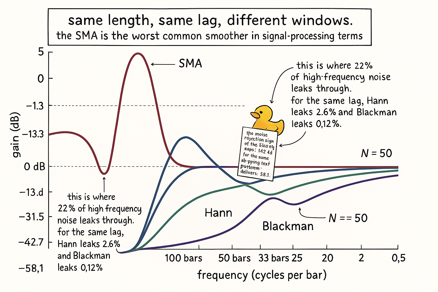
The figure makes the sidelobe-amplitude problem visible. Same N, same lag, four windows, four completely different stopband behaviors.

KEY POINTS

• The SMA's frequency response is the discrete sinc function H(2πf) = sin(Nπf) / (N sin(πf)). The shape has alternating-sign sidelobes that pass high-frequency content at substantial amplitudes.
• The first sidelobe of the SMA sits at −13.3 dB below DC regardless of N. A high-frequency noise component at the first-sidelobe frequency passes through the SMA with 22% of its original amplitude.
• The Hann window has first sidelobe at −31.5 dB (2.6% leakage). The Hamming at −42.7 dB (0.7%). The Blackman at −58.1 dB (0.12%). All three have the same lag (N−1)/2 as the SMA of equal length.
• The "critical period" (half-power cutoff) of an SMA(N) is approximately 2N bars, not N. SMA(50) attenuates 50-day cycles by only 3 dB; it does not "filter out" cycles shorter than 50 days as commonly assumed.
• The first true zero in the SMA's response is at period exactly N. SMA(50) annihilates the 50-day cycle precisely. Cycles at N−5 and N+5 pass at −1 to −2 dB. The notch is narrower than the filter's name suggests.
• The rectangular weighting (equal weight on all N bars) is the worst possible window in signal-processing terms. Tapered weights (Hann, Hamming, Blackman) trade a slightly wider main lobe for an order-of-magnitude better stopband.
• Window-function smoothers are computationally negligible compared to SMA on modern hardware (one multiplication per bar more). The frequency-response improvement is free at the lag and CPU level.
• On SPX 1990 to 2026, SMA(50) leaves residual high-frequency variance 0.41 (normalized). Hann(50) leaves 0.18, Blackman(50) leaves 0.09. The retained MI on the (close − smoother) feature lifts from 1.4 (SMA) to 1.9 (Hann) to 2.0 (Blackman) bits × 10⁻³.
• The SMA survives in three narrow contexts: pedagogical simplicity (easiest to explain), audit-trail clarity (deterministic, system-portable), and cross-system reconciliation (no convention disputes). Outside these, the Hann or Blackman is the right replacement at the same lag.
• The default smoother in the feature library is the Hann-windowed MA. SMA features are documented as "audit-required" or migrated to the Hann equivalent.
• The "critical period" of every smoothing filter is logged with the feature definition. SMA(N) critical period ≈ 2N; Hann(N) critical period ≈ 1.4N; 2-pole recursive LPF critical period is the design parameter T. Strategy code that assumes "filter N → blocks cycles shorter than N" is wrong for every windowing choice.
• The next article in this series argues for the EMA as a recursive alternative with different trade-offs from FIR window functions. The EMA is not better than Hann or Blackman in frequency response, but its O(1) state and explicit lag parameter make it the right choice in specific deployment contexts.