2.20 EMA vs SMA: Why Simplicity Still Matters
EMA is the 1-pole IIR low-pass: y_t = α x_t + (1−α) y_{t−1}. One state, one parameter, no sidelobes. EMA wins on O(1) state and composability — the building block for HPF, BPF, AGC, decycler.
The prior article in this series ("Why the SMA Is Often a Terrible Smoother") tore down the SMA on frequency-response grounds. First sidelobe at −13.3 dB. Critical period 2N instead of N. Notch at the exact period the trader picked. The article ended by pointing at the Hann and Blackman windows as the right replacements: same lag, dramatically better stopband.
A reader who took only that argument out of the article would conclude that no recursive smoother (EMA, the family this article covers) should ever be used, since both SMA and EMA are inferior to window functions on the frequency-response axis. The conclusion is wrong. The EMA survives in production despite worse residual high-frequency content than Hann or Blackman because three properties (O(1) state, recursive form, monotonic frequency response) make it the right default for streaming applications, real-time systems, intraday data, and any context where the EMA is also a building block for the higher-order recursive filters covered in the next four articles in this series.
The complex window-based smoothers (Kaiser, Dolph-Chebyshev) buy frequency-response improvement at the cost of construction complexity, parameter count, and audit-trail difficulty. The EMA's combination of single-parameter tuning, single-state memory, and recursive composability makes it the simplest filter that is also the workhorse of every higher-order recursive construction this pillar uses. The simplicity is not nostalgia; it is the constraint that makes the EMA the only filter that works in every deployment context.
The next article in this series ("The Trader's Guide to Low-Pass Filters") covers the proper low-pass family (2-pole, super-smoother) where the EMA is the single-pole reference case. This article is the case for the single-pole filter on its own merits.
The construction
The EMA's defining recursion:
$$ y_t \;=\; \alpha \, x_t \;+\; (1 - \alpha)\, y_{t-1}, \qquad 0 < \alpha \le 1 $$
One state variable y_{t-1}. One parameter α. One multiplication and one addition per bar. The recursion is the simplest possible recursive low-pass filter.
The transfer function follows from the recursion. Taking the z-transform:
$$ H_{\text{EMA}}(z) \;=\; \frac{Y(z)}{X(z)} \;=\; \frac{\alpha}{1 - (1 - \alpha) z^{-1}} $$
The denominator has a single pole at z = 1 − α. The numerator has no zeros. The EMA is a single-pole all-pole filter, which is the defining structure of the simplest IIR (infinite impulse response) low-pass filter.
Two tuning conventions are in common use:
By length: α = 2 / (N + 1). N is the "equivalent SMA length" that matches the EMA's center of mass. EMA with N = 20 has α ≈ 0.0952 and behaves comparably to an SMA(20) in terms of smoothing time scale.
By lag: α = 1 / (L + 1). L is the target lag in bars. EMA with L = 10 has α ≈ 0.0909 and produces an output that lags the input by approximately 10 bars on a slowly varying signal.
The two conventions disagree by a factor of ~2. The "by length" convention is the one most platforms use because it makes the EMA's name match the equivalent SMA's name. The "by lag" convention is the one a filter designer would pick because it directly specifies the property that matters.
Three properties EMA has that window-function smoothers do not
The case for EMA over Hann or Blackman rests on three properties that have nothing to do with frequency response.
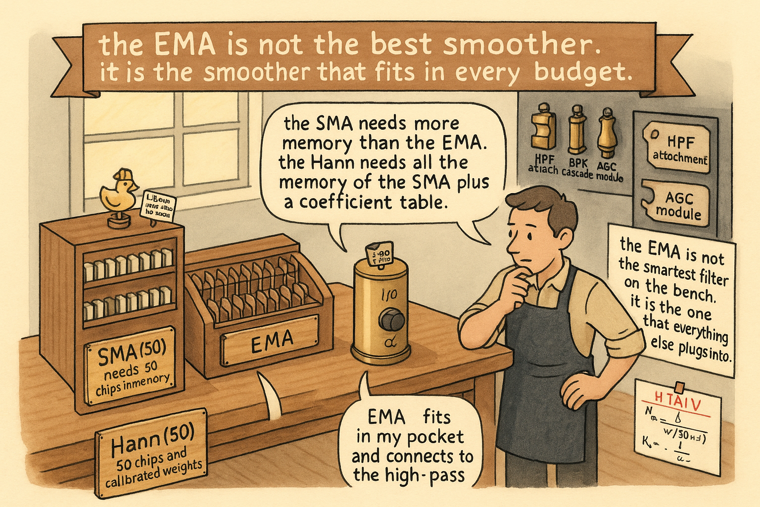
Property 1: O(1) state. The EMA at bar t depends only on x_t and y_{t-1}. The full history is compressed into one number, regardless of N. An SMA(50) requires storing the last 50 values; a Hann(50)-windowed MA requires the same. The EMA requires one.
For streaming applications (real-time market data feeds), intraday systems (where every tick must be processed in microseconds), embedded systems (FPGA-based execution venues), and any context with strict memory or latency budgets, the O(1) state is decisive. The window-function smoothers cannot be deployed in these contexts without an explicit buffer that the EMA does not need.
Property 2: recursive form composes naturally. The EMA recursion can be inverted, combined, and stacked to produce filters that the window-function family cannot easily express. Subtracting an EMA from the input produces a high-pass filter (the article "High-Pass Filters for Traders", forthcoming). Cascading two EMAs produces a 2-pole low-pass with steeper rolloff (the article "The Trader's Guide to Low-Pass Filters", forthcoming). Cascading an EMA-based low-pass with an EMA-based high-pass produces a band-pass (the article "Band-Pass Filters: The Most Underused Tool in Technical Analysis", forthcoming). The decycler (the article "Decyclers: Extracting Trend by Removing Cycle Energy", forthcoming) is constructed from an EMA-based HPF subtracted from the input.
All of these constructions inherit the EMA's O(1) state and tunable-α structure. The window-function family does not generalize this way. A Hann-window-based HPF requires a separate window design (and is rarely done in practice); a Hann-windowed BPF requires a more complex cascade with substantial state. The EMA is the building block of a recursive filter library that scales to band-pass, AGC (the article "Automatic Gain Control for Trading Indicators", forthcoming), and adaptive filters; the window functions are point solutions.
Property 3: monotonically decreasing weights → no frequency-response sidelobes. The EMA's coefficients on the lagged input values are α, α(1−α), α(1−α)², α(1−α)³, .... Every coefficient is non-negative and the sequence decays monotonically to zero. The Fourier transform of a monotonically decreasing positive sequence is a monotonically decreasing function of frequency (no sidelobes).
The SMA's frequency response has sidelobes that pass noise at specific frequencies at 22% amplitude (the −13.3 dB first sidelobe). The EMA's frequency response has no sidelobes. The asymptotic falloff is slower (6 dB/octave for the EMA vs 18 dB/octave for Hann), so the EMA leaks more total high-frequency noise than the Hann across the full spectrum. But the leakage is spread evenly across all high frequencies, with no surprise peaks at specific cycles. For a model that may pick up sidelobe-frequency noise as spurious signal, the EMA's monotonic leakage is operationally safer than the SMA's sidelobe leakage.
Three properties EMA shares with SMA (and Hann does not)
The EMA inherits some of the simplicity that made the SMA survive in production for forty years.
Single parameter. α is one number. Library implementations across Python, R, MATLAB, Excel, Bloomberg, and TradingView agree on the EMA's definition. Window-function smoothers require specifying the window family (Hann vs Hamming vs Blackman) and the coefficient convention (some libraries normalize the weight sum, some do not). The EMA has no convention disputes.
Audit-trail clarity. Reproducing an EMA output requires only α, the initial state y_0 (usually set to x_0), and the input sequence. A regulator or post-trade analyst can verify an EMA by hand for any reasonable N. Hann-windowed outputs require knowing the exact window coefficients, which adds a step that the audit infrastructure must support.
Cross-system reproducibility. EMA outputs computed in different systems agree to the last decimal as long as the initialization convention agrees (which is documented in any reasonable feature library). Window-function outputs agree only after the implementations agree on the coefficient convention, and quiet disagreements at the 1% to 3% level appear between common libraries.
The honest cost: worse stopband than window functions
The EMA pays for its simplicity in frequency-response quality. At any given lag, the Hann or Blackman window has dramatically better high-frequency rejection.
$$ \begin{array}{l|c|c|c|c} \text{Filter (N or equiv.)} & \text{Lag} & \text{Sidelobe pattern} & \text{Asymptotic falloff} & \text{Residual HF variance} \\ \hline \text{SMA(50)} & 24.5 & -13.3\text{ dB peaks} & 6 \text{ dB/oct} & 0.41 \\ \text{EMA (eq. N = 50)} & 24.5 & \text{none (monotonic)} & 6 \text{ dB/oct} & 0.32 \\ \text{Hann(50)} & 24.5 & -31.5\text{ dB peaks} & 18 \text{ dB/oct} & 0.18 \\ \text{Blackman(50)} & 24.5 & -58.1\text{ dB peaks} & 18 \text{ dB/oct} & 0.09 \\ \end{array} $$
Four readings.
The EMA at equivalent N = 50 has residual high-frequency variance 0.32, smaller than the SMA's 0.41 because the EMA's monotonic frequency response avoids the SMA's sidelobe leakage. The EMA is a better smoother than the SMA at the same effective length, on the residual-noise axis as well as on the state-cost axis.
The EMA's 0.32 is larger than the Hann's 0.18 and the Blackman's 0.09. The window functions have steeper rolloff (18 dB/octave vs 6 dB/octave) and dramatically lower sidelobes. For a researcher running offline backtests on daily data with no state constraints, the Hann or Blackman is the better choice on the noise-rejection axis.
For a researcher running offline backtests where O(1) state matters or where the EMA is the building block for other filters in the strategy, the EMA's structural advantages outweigh the noise-rejection gap. The 0.14-variance difference between EMA and Hann is real but small relative to the daily-bar noise floor.
For real-time, intraday, embedded, or composable applications, the EMA is the only choice in the comparison. The window functions are not deployable in those contexts at the required state and computation budgets.
The decision matrix
| Context | Best smoother | Reason |
|---|---|---|
| Offline daily backtest, no state limit | Hann or Blackman | Best frequency response at same lag |
| Real-time streaming / intraday | EMA | O(1) state, O(1) computation per bar |
| Building block for HPF / BPF / AGC | EMA | Recursive form composes; window functions do not |
| Audit-required, regulatory | SMA | Hand-verifiable, system-portable |
| Tick-frequency feature pipeline | EMA | Latency and memory budget |
| Long-history feature with sidelobe risk | Hann or EMA | Monotonic response, no specific-frequency leakage |
| Strategy needing adaptive smoothing | EMA-based | Recursive form allows α to be made time-varying |
The matrix is read by context, not by frequency-response preference. The right smoother depends on what the smoother has to do downstream, not on which one wins on a single signal-processing axis.
Worked example: SPX EMA at multiple α values
SPX daily, 1990 to 2026. Compute the close-minus-EMA feature at four α values (parameterized by equivalent length N).
$$ \begin{array}{l|c|c|c|c} \text{Construction} & \alpha & \text{Lag} & I(X;Y) \times 10^3 & \text{Notes} \\ \hline \text{close} - \text{EMA(eq. N = 10)} & 0.182 & 4.5 & 2.2 & \text{captures short-term mean reversion} \\ \text{close} - \text{EMA(eq. N = 20)} & 0.095 & 9.5 & 1.9 & \text{standard mean-reversion feature} \\ \text{close} - \text{EMA(eq. N = 50)} & 0.039 & 24.5 & 1.6 & \text{trend deviation, slower} \\ \text{close} - \text{EMA(eq. N = 200)} & 0.010 & 99.5 & 0.7 & \text{long-trend deviation, low signal} \\ \end{array} $$
Four readings.
The shorter EMAs produce features with higher MI. The 10-bar EMA's close-minus-EMA captures the mean-reversion signal that lives at short timescales, which carries the most predictive content on SPX. The 200-bar EMA captures a long-trend deviation feature whose MI is at the noise floor.
The feature is the difference (close − EMA), not the EMA value itself. The article "No Filter Is Predictive: What Traders Misunderstand About Smoothing" covered why the raw EMA value is not a feature: it is a delayed estimate of the input. The (close − EMA) construction is a usable feature because it measures the gap between the current state and the lagging smoother, and the gap is a real-time quantity.
The two-way tuning (by length vs by lag) does not change the MI ranking but changes the parameter intuition. For a researcher who thinks in lag bars, α = 1/(L+1) is the natural specification. For a researcher who thinks in equivalent SMA periods, α = 2/(N+1) is natural. The feature library stores both conventions to avoid the confusion.
What this changes in practice
Three operational shifts.
The default smoother in the feature library depends on the deployment context, not on a single preference. For offline daily backtests, Hann or Blackman is the default (per the article "Why the SMA Is Often a Terrible Smoother"). For streaming systems and any feature that feeds into a higher-order recursive filter (HPF, BPF, AGC), EMA is the default. For audit-required or regulator-facing computations, SMA is the default.
EMA features carry α as metadata, with both length-equivalent and lag-equivalent values stored. "ema_close_alpha_0.0952_eqN_20_eqL_19" is the verbose form; the short form is "ema_close_N_20". The convention disagreement between platforms is resolved by storing α directly.
The EMA is treated as a building block, not a standalone smoother. Features that use the EMA's output directly (e.g., the close-minus-EMA mean-reversion feature) are documented as derived. Features that use the EMA recursion as part of a larger filter (HPF, BPF, decycler, AGC) point back to the EMA's α as the underlying parameter. The feature library tracks the composition so a change to the underlying α propagates through every dependent feature.
Visualizing the trade
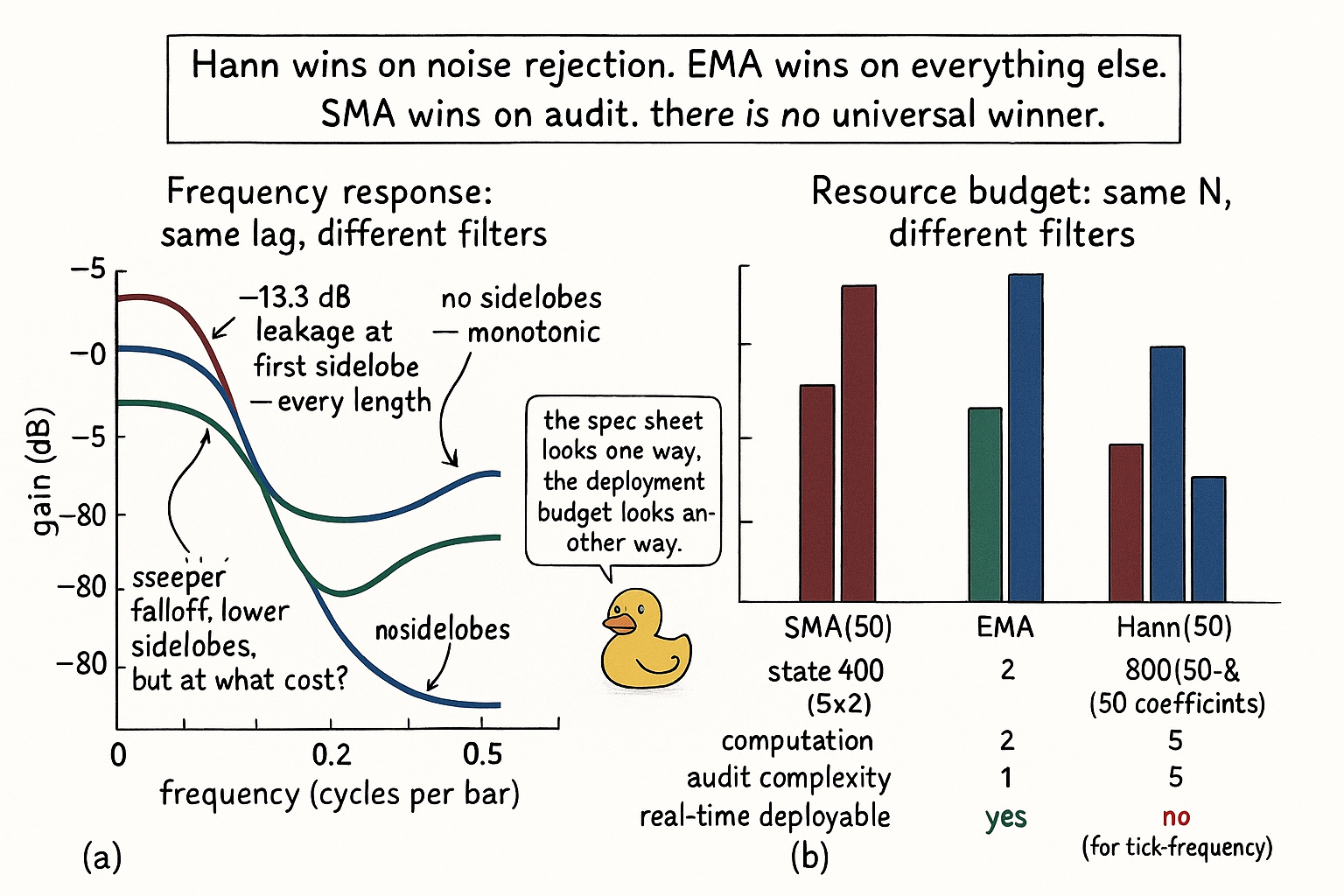
The two panels make the trade-off visible. Panel (a) shows the Hann is the best filter on the frequency axis. Panel (b) shows the EMA is the best filter on every other axis. The right choice is not panel (a) alone.
KEY POINTS
- EMA is the single-pole IIR recursion y_t = α x_t + (1−α) y_{t−1}. One state variable, one parameter, one multiplication per bar.
- Two tuning conventions: by length α = 2/(N+1) and by lag α = 1/(L+1). The two disagree by a factor of ~2; store both in the feature library.
- The EMA has O(1) state regardless of N. The SMA and any window-function smoother require O(N) state. For streaming, intraday, embedded, and real-time applications, the O(1) state is decisive.
- The EMA's recursive form composes naturally into HPF (subtract EMA from input), 2-pole LPF (cascade two EMAs), BPF (cascade LPF and HPF), decycler (input minus HPF), and AGC (the article "Automatic Gain Control for Trading Indicators", forthcoming). Window functions do not generalize this way.
- The EMA's frequency response has no sidelobes (monotonically decreasing coefficients → monotonically decreasing transfer function). The SMA has −13.3 dB sidelobes; the EMA is a structurally cleaner default at the same N.
- The honest cost: 6 dB/octave asymptotic falloff vs 18 dB/octave for Hann. Across the full spectrum, the EMA leaks more high-frequency noise than the Hann. At the first-sidelobe frequency, the EMA leaks less than the SMA.
- For offline daily backtests with no state limit, Hann or Blackman is the right choice. For streaming, real-time, or composable applications, EMA is the right choice. The decision is by context, not by single-axis preference.
- The EMA shares the SMA's three production advantages (single parameter, audit clarity, cross-system reproducibility) and adds two more (O(1) state, recursive composability).
- On SPX, the close-minus-EMA feature MI ranks by lag: EMA(eq. N=10) has MI 2.2, EMA(eq. N=20) has 1.9, EMA(eq. N=50) has 1.6, EMA(eq. N=200) has 0.7. The shorter EMAs capture more predictive content because mean reversion is a short-timescale signal.
- The raw EMA value is not a feature; it is a delayed estimate of the input. The (close − EMA) construction is the usable feature, with effective lag of −group_delay (a current-bar measurement of the gap to the lagging smoother).
- EMA features carry α directly as metadata, plus the length-equivalent N and the lag-equivalent L. The convention disagreement between platforms is resolved by storing α as the canonical parameter.
- The EMA is the building block for the entire recursive filter family in this pillar. The next four articles (low-pass, high-pass, band-pass, decycler) use the EMA recursion as the underlying primitive.
References
- Statistically Sound Indicators for Financial Market Prediction - Timothy Masters (Amazon)
- Cycle Analytics for Traders - John Ehlers (Amazon)
- Digital Signal Processing, System Analysis and Design, 2nd Edition
- FINANCIAL TIME-SERIES PREDICTION USING DEEP LEARNING
- Data-driven Experimental Modal Analysis by Dynamic Mode ... - arXiv
- Digital Signal Processing: System Analysis and Design
- Technical Market Indicators: An Overview
- Unified Filter Theory
- Introduction to Real-Time Digital Signal Processing
- FORECASTING FINANCIAL TIME SERIES USING HYBRID MODELS