2.29 Automatic Gain Control for Trading Indicators
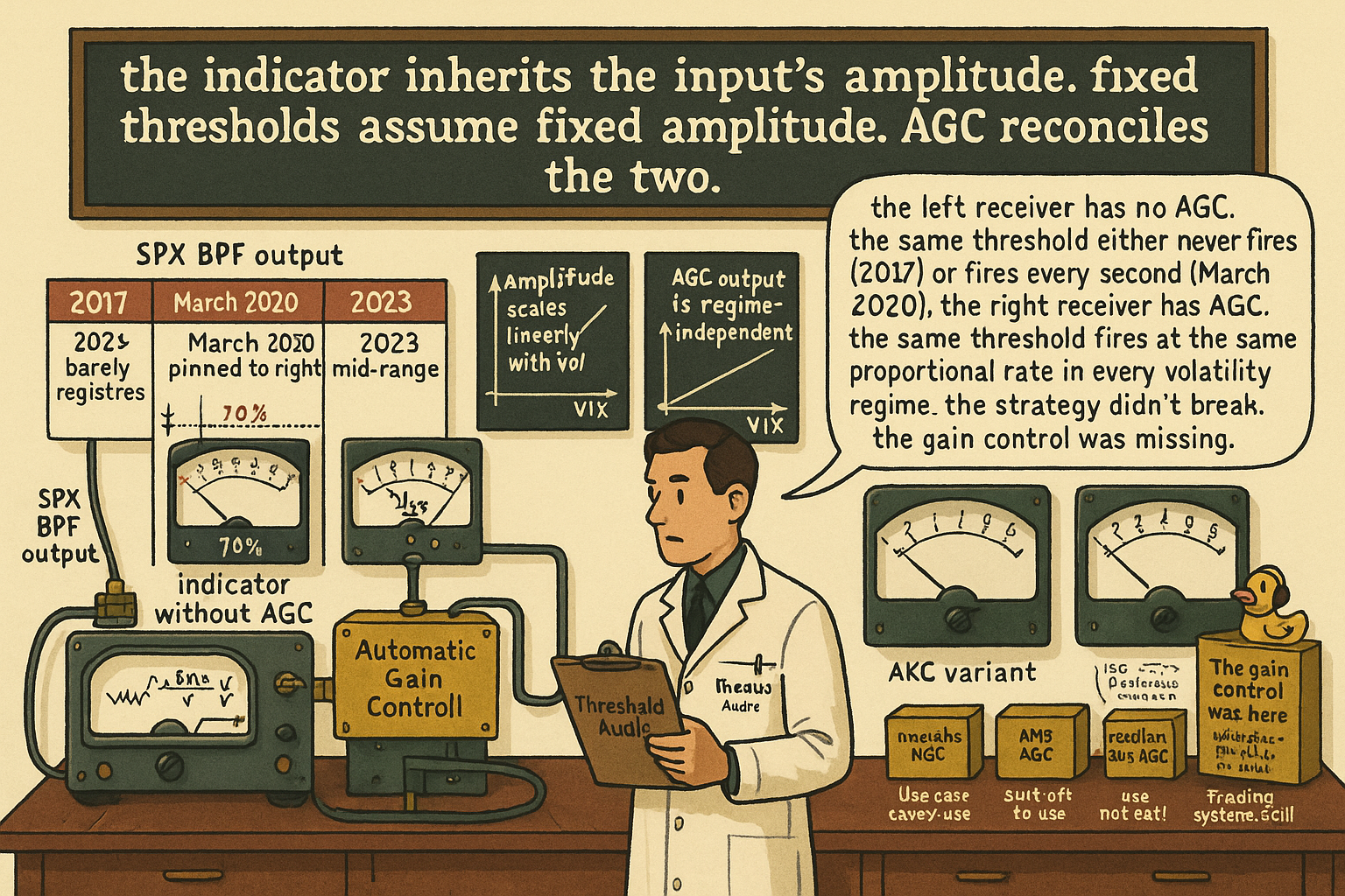
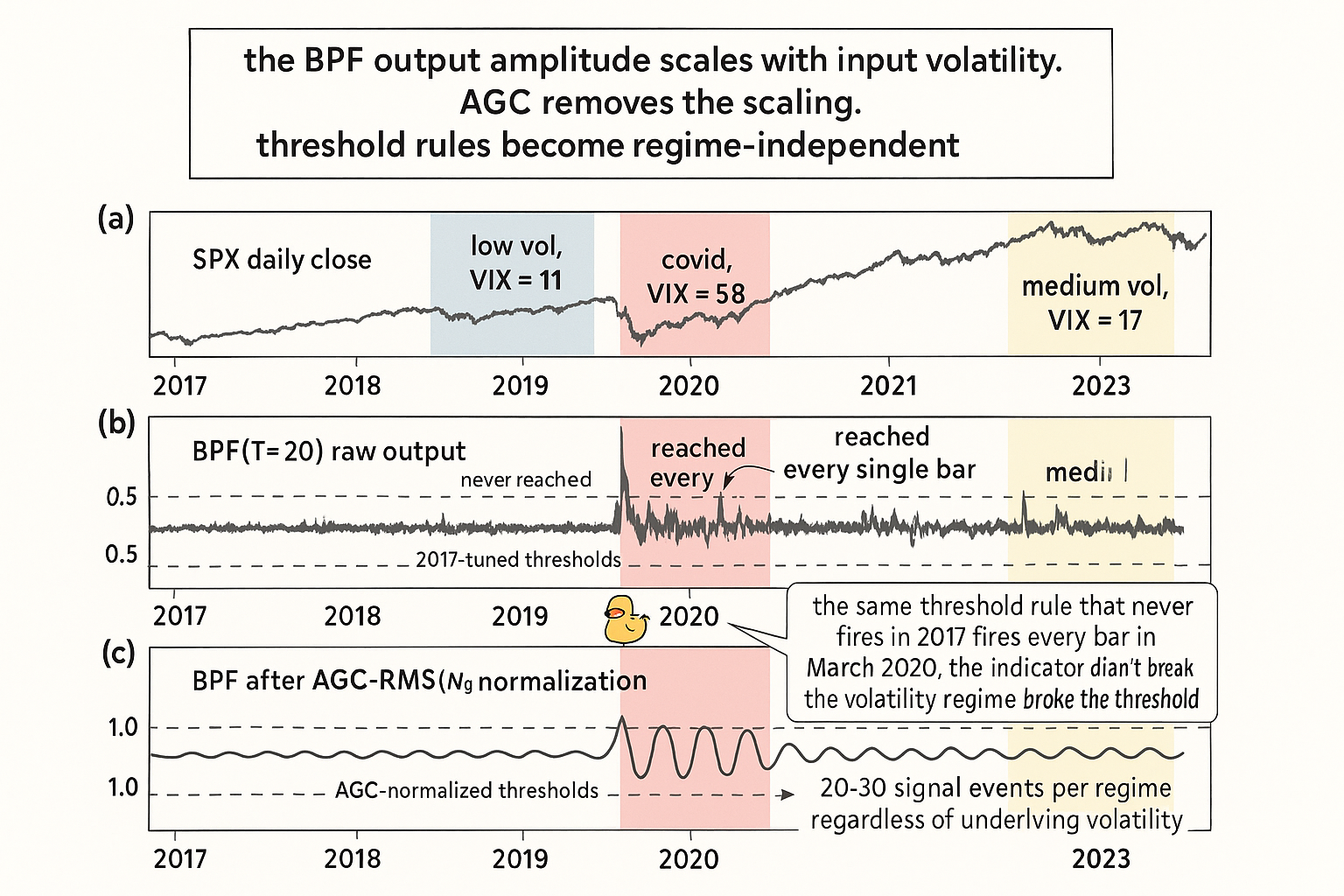
Indicators inherit the input's amplitude. BPF on SPX swings ±0.4% in 2017 and ±3.1% in March 2020. AGC rescales continuously so thresholds become regime-independent. The fix is one pipeline stage.
A trader tunes an RSI(14) mean-reversion strategy on SPY 2017 data. The rule: short when RSI crosses above 70, cover at 50. The backtest shows 22 winning trades, 4 losing trades, Sharpe 1.6 over the calendar year. The trader ships the strategy and runs it through March 2020. RSI hits 70 on March 2, 75 on March 4, 80 on March 6, and stays above 70 for eleven consecutive sessions while SPY drops from 311 to 219. By the time RSI finally drops back below 70 on March 23, the strategy has lost three months of accumulated profit on a single position.
The trader concludes the strategy "needs different thresholds for high-vol regimes" and adds a VIX filter that disables the strategy when VIX > 30. The patch works but the underlying problem is not fixed. The same diagnosis applies to BPF outputs, MACD readings, close-minus-MA distances, Stochastic levels, and every other oscillator-based threshold rule. The indicator's output amplitude scales with the input's volatility. A threshold tuned for one volatility regime is wrong for any other regime by construction.
Automatic gain control fixes the problem at the structural level. Instead of applying fixed thresholds to an indicator whose amplitude varies with volatility, normalize the indicator's amplitude continuously so the output stays in a fixed range regardless of the input regime. Threshold rules applied to the AGC output are regime-independent. The same RSI > 70 rule that worked in 2017 works in March 2020 because the AGC has rescaled both periods to a comparable amplitude range.
The article "Why ATR Normalization Is More Than a Volatility Trick" gave the structurally optimal scaling for price-unit features (divide by ATR with the √k factor). The article "Taming Indicator Tails with Sigmoid Transforms" gave the bounded-but-monotone scaling for heavy-tailed features (sigmoid into the linear region). AGC is the third member of this family: bounded, regime-adaptive, designed for indicators that need consistent visual amplitude across all market conditions. This article gives the constructions, the structural caveats, and the operational discipline. The next article in this series ("Dominant Cycle Estimation Without Astrology") covers how AGC enables stable cycle measurements across regimes.
The structural problem
A linear filter applied to price preserves the price's amplitude in its output. For an SPX BPF centered at T = 20:
$$ y_{\text{BPF}}(t) \;\approx\; A_{\text{cycle}}(t) \cdot \cos(\omega t + \phi) $$
The output amplitude A_cycle(t) is proportional to the underlying cycle amplitude of the input. When SPX cycles 1% peak-to-trough, the BPF output ranges in ±0.5%. When SPX cycles 6% peak-to-trough, the BPF output ranges in ±3%. A trader who set a "buy when BPF < −0.5" threshold based on 2017 data triggers continuously in March 2020 and never triggers in summer 2023.
The same property holds for every linear indicator covered in the prior articles in this series. The article "The Frequency Response of Trading Indicators" gave the universal framework: a linear filter has unit gain (or some constant gain) at its passband frequency. The output amplitude at the passband is the input amplitude multiplied by the gain. Threshold rules that ignore the regime-dependent input amplitude are reading the indicator wrong by construction.
Three options to fix this. Option 1: change the threshold for each regime (regime-detection layer + threshold lookup). Operationally fragile. Option 2: replace the threshold rule with a relative comparison (current value vs rolling mean of the same indicator). Better, but still depends on the rolling window length. Option 3: rescale the indicator's amplitude continuously to a fixed range. This is the AGC approach.
The basic AGC construction
The simplest AGC normalizes by the rolling maximum absolute value:
$$ y_{\text{AGC}}(t) \;=\; \frac{x(t)}{\max_{0 \le i < N} |x(t-i)|} $$
The output is bounded in [-1, 1] by construction. The denominator is the largest absolute value the indicator has reached in the rolling window. The current value, divided by this maximum, places the current reading on a [-1, 1] scale relative to the window's extremes.
For an SPX BPF output: in March 2020 the window's max is approximately 3% (the largest BPF swing). The current BPF value of −2% becomes (−2/3) = −0.667 after AGC. In summer 2023 the window's max is approximately 0.4%. The same proportional cycle position produces the same AGC value of approximately −0.667 even though the raw BPF value is now −0.27%. The AGC output is the cycle's relative position within the current regime, not its absolute amplitude.
Threshold rules on the AGC output become regime-independent. "Buy when AGC(BPF) < −0.7" fires when the BPF reaches 70% of its recent peak excursion, whether the recent peak excursion is 3% or 0.4%.
The RMS-based AGC
Max-abs normalization has one structural flaw: it is dominated by the single largest outlier in the window. One news-day spike contaminates the denominator for N bars. The "even better sine wave" construction uses an RMS-based normalization that distributes the influence across all bars in the window:
$$ y_{\text{AGC-RMS}}(t) \;=\; \frac{x(t)}{\sqrt{\frac{1}{N} \sum_{i=0}^{N-1} x(t-i)^2}} $$
The denominator is the rolling RMS (root mean square) of the indicator's absolute amplitude. The output is centered at zero with approximately unit-variance scaling. Unlike max-abs, the RMS averages the squared amplitudes across the window, so a single outlier contributes 1/N of its squared value rather than fully determining the denominator.
The RMS AGC output is not strictly bounded by [-1, 1] (a value at 3σ amplitude registers as +3 after RMS normalization), but it is centered on zero with consistent scale across regimes. Threshold rules use multiples of unit amplitude: "buy when AGC-RMS < −1.5" maps to "buy when current indicator is 1.5x its recent RMS amplitude on the negative side."
The choice between max-abs and RMS depends on the indicator. For BPF outputs and other oscillators with bounded natural amplitude, max-abs gives a cleaner [-1, 1] bounded output. For indicators that occasionally produce large spikes (close-minus-MA at major turning points, momentum during news days), RMS is more stable.
Comparison to alternative scaling methods
Five scaling approaches cover the indicator-normalization space. Each has structural trade-offs.
$$ \begin{array}{l|c|c|c} \text{Method} & \text{Output range} & \text{Outlier sensitivity} & \text{Best for} \\ \hline \text{Max-abs AGC} & \text{[-1, 1] strict} & \text{High (single outlier dominates)} & \text{Bounded oscillators, BPF} \\ \text{RMS AGC} & \text{Centered, scale 1} & \text{Moderate (quadratic)} & \text{Indicators with occasional spikes} \\ \text{Median-abs AGC} & \text{[-k, k] typical} & \text{Low (robust)} & \text{Heavy-tailed indicators} \\ \text{Z-score} & \text{Centered, scale 1} & \text{High (mean and std)} & \text{Approximately Gaussian indicators} \\ \text{Robust z-score (median, MAD)} & \text{Centered, scale ~1} & \text{Low} & \text{Heavy-tailed indicators} \\ \text{Percentile rank} & \text{[0, 1] strict} & \text{Low} & \text{Indicators where rank matters more than magnitude} \\ \text{Sigmoid (tanh)} & \text{(-1, 1) asymptotic} & \text{Low} & \text{Heavy tails, see "Taming Indicator Tails with Sigmoid Transforms"} \\ \text{ATR normalization} & \text{Scaled by ATR} & \text{Moderate} & \text{Price-unit features, see "Why ATR Normalization Is More Than a Volatility Trick"} \\ \end{array} $$
Eight methods. The choice depends on the indicator's structural properties.
For cycle-mode indicators (BPF outputs, Hilbert sine, sine-wave indicator), max-abs AGC or RMS AGC is the standard choice. The output is naturally bounded by the cycle's amplitude, so max-abs preserves the [-1, 1] interpretation. For indicators with rare outliers, RMS or median-abs AGC gives a more stable denominator.
For statistical features that approximate Gaussian behavior, z-score is appropriate. For heavy-tailed features (most real trading features), robust z-score using median and MAD is the better choice. The article "Why the Median Often Beats the Mean in Trading Features" detailed the robust-statistics argument.
For price-unit features (price minus MA, momentum), ATR normalization is structurally optimal because it accounts for the random-walk √k factor in the variance scaling. The article "Why ATR Normalization Is More Than a Volatility Trick" detailed the construction.
Structural issues with AGC
Three issues that show up when AGC is applied without care.
Issue 1: window length tradeoff. Too short (N < 10) makes the denominator noisy and the AGC output unstable. Too long (N > 100) makes the AGC slow to adapt to regime changes. The article "How to Think About Indicator Lag Before Backtesting" frames this as a lag-budgeting question: the AGC denominator carries the lag of an N-bar smoother on the absolute-value channel.
For SPX daily, N = 40 to N = 100 is the typical operational range. Shorter windows produce visible jitter in the AGC output. Longer windows lag the regime change so the AGC output continues to use 2017-style scaling for 2020-style price action for several weeks after the regime shift.
Issue 2: max-abs is dominated by outliers. A single news-day spike sets the denominator for N bars. After the spike, the AGC output is compressed (everything looks smaller than it is) until the spike rolls out of the window. Solutions: switch to RMS or median-abs, or apply a Hampel pre-filter (covered in "Why Median Filters Are Useful for Volume and Outliers") to remove spikes from the absolute-value series.
Issue 3: memory effects. The AGC denominator is a function of past values. After a true regime shift (sustained volatility expansion), the denominator takes N bars to fully reflect the new regime. During the transition, the AGC output gives mixed-regime readings that are not directly comparable to either the old or new regime's typical readings.
The mitigation: use a faster AGC window during anticipated regime transitions (e.g., during VIX expansion phases), and a slower window during stable regimes. The dual-window approach is operationally simple but adds complexity to the indicator pipeline.
Robust AGC hybrids
Three hybrid constructions improve on the basic AGC for specific failure modes.
Hybrid 1: median-abs AGC. Replace the max-abs denominator with the rolling median of |x|. The median is robust to single-spike contamination (covered in "Why Median Filters Are Useful for Volume and Outliers"), so the AGC denominator is stable even when the indicator has occasional outlier readings.
$$ y_{\text{AGC-med}}(t) \;=\; \frac{x(t)}{k \cdot \text{median}_N(|x(t-i)|)}, \qquad k \approx 1.4826 \text{ (for Gaussian scale equivalence)} $$
The factor k makes the median-abs denominator approximately equal to one standard deviation for Gaussian inputs. The construction is the most robust of the AGC family.
Hybrid 2: EMA-of-abs AGC. Replace the rolling max-abs with an EMA of |x|. The denominator becomes a smoothly updating estimate of the typical absolute amplitude rather than a hard maximum:
$$ \hat{a}(t) \;=\; \alpha \cdot |x(t)| + (1 - \alpha) \cdot \hat{a}(t-1), \qquad y_{\text{AGC-EMA}}(t) \;=\; \frac{x(t)}{\hat{a}(t)} $$
The output is unbounded (extreme values produce extreme AGC readings) but the denominator transitions smoothly across regimes. The EMA's lag is the standard EMA lag at the equivalent lookback (covered in "The Hidden Cost of Every Moving Average: Lag").
Hybrid 3: Hampel-pre-filtered AGC. Apply a Hampel filter to the indicator output first to remove outlier spikes, then apply standard AGC to the cleaned series. The AGC denominator is not contaminated by spikes because the spikes are removed before scaling.
The choice among hybrids depends on the data class. For volume-weighted indicators or true-range-based indicators, Hampel-pre-filtered AGC is the default (the underlying data has known outlier structure). For BPF cycle outputs on clean price data, max-abs or RMS AGC is sufficient. For long-tail indicators (close-minus-MA at turning points), median-abs AGC is the most robust.
Worked example: SPX BPF across regimes
SPX daily. Apply a BPF(T=20, δ=0.3) and compare four AGC variants across three volatility regimes.
$$ \begin{array}{l|c|c|c|c} \text{Period} & \text{VIX avg} & \text{BPF raw amplitude} & \text{No AGC} & \text{AGC output range} \\ \hline \text{Calendar 2017} & 11.1 & \pm 0.4\% & \text{[-0.4\%, 0.4\%]} & \text{[-1, 1]} \\ \text{Mar 2020 (covid)} & 57.7 & \pm 3.1\% & \text{[-3.1\%, 3.1\%]} & \text{[-1, 1]} \\ \text{Calendar 2023} & 17.0 & \pm 0.9\% & \text{[-0.9\%, 0.9\%]} & \text{[-1, 1]} \\ \end{array} $$
The raw BPF amplitude varies by a factor of approximately 8 across the three regimes. A "buy when BPF < −0.5%" rule fires 100% of the time in March 2020 (every bar) and 0% of the time in 2017 (the BPF never reaches −0.5% in that period). After AGC normalization, the same proportional cycle position produces the same AGC value in all three regimes. A "buy when AGC < −0.7" rule fires at structurally comparable points across all three periods.
Now compare the AGC variants on the same data.
$$ \begin{array}{l|c|c|c|c} \text{AGC variant} & \text{Bounded?} & \text{Outlier impact} & \text{Lag to regime shift} & \text{Best use} \\ \hline \text{Max-abs(N=60)} & \text{[-1, 1]} & \text{High (single spike sets denom 60 bars)} & \text{Slow (denom fixed at max)} & \text{Clean oscillators} \\ \text{RMS(N=60)} & \text{Soft (typically [-3, 3])} & \text{Moderate (quadratic)} & \text{Medium} & \text{Occasional spikes} \\ \text{Median-abs(N=60)} & \text{Soft (typically [-3, 3])} & \text{Low} & \text{Medium} & \text{Heavy-tailed indicators} \\ \text{EMA-of-abs(} \alpha{=}0.04) & \text{Unbounded} & \text{Moderate (decays)} & \text{Fast} & \text{Real-time regime adaptation} \\ \end{array} $$
The trade-off: max-abs gives the cleanest bounded output but is the slowest to adapt to regime shifts. EMA-of-abs adapts fastest but produces unbounded output. RMS and median-abs sit in the middle, with median-abs being the most robust choice for indicators with heavy-tailed behavior.
For most cycle-mode trading applications, RMS(N=60) or median-abs(N=60) is the default. Max-abs is reserved for indicators that need strict [-1, 1] bounds for downstream consumption (visual display, fixed-bound classifiers).
Where AGC fails
Four scenarios where AGC produces misleading or unhelpful output.
Scenario 1: indicators with no natural zero. AGC assumes the indicator is centered at zero (positive and negative excursions roughly balanced). For indicators with DC offset (raw price, cumulative sums), AGC produces garbage. Apply a centering operation (close-minus-MA, HPF) first to remove the DC, then AGC.
Scenario 2: when absolute magnitude matters. AGC throws away the absolute amplitude information by construction. If the strategy needs to know "is the current cycle large or small in absolute terms," AGC removes the answer. Use a parallel raw-amplitude channel alongside the AGC channel.
Scenario 3: regime-shift outliers. A sudden volatility expansion that lasts longer than N bars causes the AGC to gradually rescale to the new regime. During the transition (first N bars of the new regime), the AGC output mixes old and new regime scales. Threshold rules during this transition are ambiguous.
Scenario 4: cross-instrument comparisons. AGC normalizes within an instrument's own volatility regime. Comparing AGC outputs across SPX and crude oil produces relative readings within each instrument's history, not directly comparable readings. For cross-instrument comparison, use a structurally cross-comparable normalization like ATR (covered in "Why ATR Normalization Is More Than a Volatility Trick") or rank-based normalization.
What this changes in practice
Five operational shifts.
Apply AGC to every threshold-based oscillator rule. The fix is one extra pipeline stage and removes the regime-dependence of fixed thresholds. RSI thresholds (70/30), BPF triggers, MACD signals all benefit from AGC normalization before the threshold is applied.
Default to RMS or median-abs AGC for production. Max-abs AGC is the textbook construction but is fragile to single outliers. RMS or median-abs gives comparable bounding with much better robustness.
Match the AGC window length to the regime persistence. For markets with rapid regime shifts (crypto, leveraged products), use shorter windows (N = 20-40). For markets with slower regime evolution (large-cap equity indices), use longer windows (N = 60-100).
Report indicator readings paired with the AGC method explicit. "RSI(14) AGC-RMS(60)" is unambiguous. "RSI(14)" without disclosure of the scaling is regime-ambiguous.
Audit existing strategies for "fixed thresholds on raw oscillator" anti-patterns. Any strategy with hardcoded threshold values on RSI, MACD, Stochastic, BPF, or any other amplitude-sensitive indicator is at risk of regime-shift breakdown. The fix is to insert AGC between the indicator and the threshold.
Decision matrix
| Use case | Recommended AGC | Reason |
|---|---|---|
| BPF cycle oscillator on equity index | Max-abs or RMS, N = 60 | Bounded output for clean visual |
| Cycle-mode features with occasional spikes | RMS, N = 60 | Quadratic robustness |
| Heavy-tailed indicators (close-minus-MA at extremes) | Median-abs, N = 60 | Robust to outliers |
| Volume-weighted indicators | Hampel pre-filter + RMS | Volume has heavy right tail |
| True-range smoothing | Hampel pre-filter + median-abs | TR spikes on news days |
| Real-time regime adaptation needed | EMA-of-abs, α = 0.05 | Fast adaptation, smooth update |
| Cross-instrument comparison | Not AGC; use ATR or rank | AGC is within-instrument only |
| Raw oscillator with DC offset | Center first (HPF), then AGC | AGC assumes zero-centered input |
| Need absolute amplitude information | AGC + parallel raw channel | AGC discards amplitude |
Anti-patterns
Five mistakes when applying AGC.
Anti-pattern 1: fixed thresholds on raw oscillator output. RSI > 70 / RSI < 30 rules are regime-dependent. Apply AGC first, then threshold.
Anti-pattern 2: using max-abs AGC on indicators with heavy-tailed behavior. A single outlier sets the denominator for N bars and compresses the AGC output. Use RMS or median-abs instead.
Anti-pattern 3: too short an AGC window. N < 10 produces noisy denominators that make the AGC output jitter independently of the underlying signal. Use N ≥ 20.
Anti-pattern 4: AGC on an uncentered indicator. AGC assumes the input is zero-centered. For DC-biased inputs (raw price, cumulative volume), AGC produces garbage. Center first with an HPF or a close-minus-MA construction.
Anti-pattern 5: cross-instrument comparison via AGC. AGC normalizes within each instrument's own history. The same AGC value on SPX and crude oil means "70% of the recent extreme in this instrument," not "comparable cycle states." Use ATR-based normalization or cross-sectional ranking instead.
Visualizing AGC
KEY POINTS
- Linear indicators preserve their input's amplitude. A BPF on SPX in 2017 (low vol) produces outputs in ±0.4%. The same BPF in March 2020 (high vol) produces outputs in ±3.1%. The 8x amplitude difference breaks any fixed-threshold rule.
- AGC continuously rescales the indicator output so the amplitude stays in a fixed range regardless of input volatility. Threshold rules on the AGC output are regime-independent.
- Basic AGC: divide the current indicator value by the rolling max of the absolute value over N bars. Output is bounded in [-1, 1].
- RMS AGC: divide by the rolling RMS instead of max-abs. Output is centered with approximately unit-variance scaling. More robust to single-spike contamination.
- Median-abs AGC: divide by the rolling median of |x|. Most robust of the AGC family, suited for heavy-tailed indicators.
- EMA-of-abs AGC: smooth recursive update of the denominator. Fastest adaptation to regime shifts, but unbounded output.
- AGC is one of three structural normalization families: AGC for oscillators, ATR for price-unit features, sigmoid for heavy-tailed indicators with bounded targets.
- Three structural issues with AGC: window length tradeoff (short = noisy, long = lagging), max-abs outlier sensitivity, memory effects during regime transitions.
- Anti-pattern: applying AGC to uncentered indicators (raw price, cumulative sums). AGC assumes zero-centered input. Apply HPF or close-minus-MA first.
- Anti-pattern: cross-instrument comparison via AGC. AGC is within-instrument only. For cross-instrument comparison use ATR or cross-sectional ranking.
- Default AGC choice for production: RMS(N=60) or median-abs(N=60) on cycle-mode indicators. Max-abs is reserved for strict [-1, 1] bounding when required.
- Existing strategies with hardcoded thresholds on raw RSI, MACD, Stochastic, BPF outputs are at structural risk of regime-shift breakdown. The fix is one pipeline stage: insert AGC before the threshold.
References
- Statistically Sound Indicators for Financial Market Prediction - Timothy Masters (Amazon)
- Cycle Analytics for Traders - John Ehlers (Amazon)
- Technical Analysis: The Role of Machine Learning in Technical Trading
- Complex Systems for Investment Management
- [Retracted] A Study of Stock Market Predictability Based on Financial
- arXiv:2504.07515v1 [astro-ph.IM] 10 Apr 2025
- The Twilight Zone: OTC Regulatory Regimes and Market Quality
- Full article: A novel deep learning model for stock market prediction
- Computer Science - arXiv
- Dynamic Asset Allocation with Asset-Specific Regime Forecasts - arXiv