2.30 Dominant Cycle Estimation Without Astrology
The dominant cycle is measurable. Autocorrelation periodogram gives a number with known precision. Elliott Wave, Gann, Bradley dates produce no falsifiable measurement. Numbers feed adaptive logic.
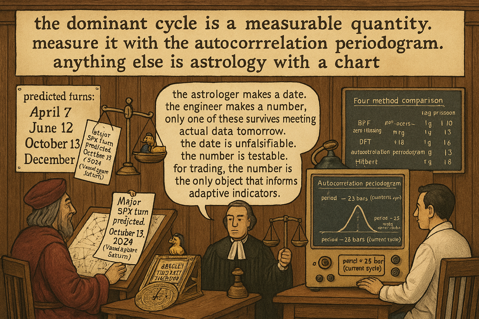
A trader reads an analyst's note predicting "a major SPX turn on October 13, 2024" based on a Bradley turn-date model derived from planetary aspects. The note presents the date with confidence and includes a chart of historical Bradley dates "marking" past turns. The trader buys puts ahead of the date. October 13 arrives. SPX closes up 0.4% on no news. The next day SPX is up another 0.6%. The trader's puts expire worthless. The analyst's next note explains that the turn "manifested as a sideways consolidation" and references a new date in November.
Two structural problems with this. First, the prediction was not falsifiable: any market behavior on October 13 can be reframed as "the turn manifesting." Second, there exists a precise, falsifiable, signal-processing-based method for estimating the current dominant cycle period of the SPX, and applying it to data through October 10 would have produced a numerical estimate ("dominant cycle currently approximately 27 bars, mid-cycle phase, no zero crossing expected in the next 5-7 bars"). The numerical estimate disagrees with the planetary forecast. The numerical estimate is testable. The planetary forecast is not.
This article gives the empirical alternative to cycle astrology. The dominant cycle period of any time series is a measurable quantity with known statistical properties. Four established methods produce numerical estimates with known precision and known failure modes. The estimates are imperfect because real market cycles are weak, time-varying, and often multiple, but the imperfection is itself a measurable property rather than a rationalization. Empirical cycle estimation is not a substitute for cycle prediction; it is a substitute for cycle hallucination.
The article "Band-Pass Filters: The Most Underused Tool in Technical Analysis" introduced the BPF zero-crossing method as a basic cycle measurement. The article "Decyclers: Extracting Trend by Removing Cycle Energy" used dominant cycle period as a parameter for the decycler. The article "Automatic Gain Control for Trading Indicators" needed a cycle-period estimate for window-length tuning. All three articles assumed access to a dominant cycle estimate. This article gives the four canonical methods, compares them on real data, and frames the structural limitations the next article in this series ("Why Market Cycles Are Evanescent") expands on.
What "dominant cycle" means precisely
A dominant cycle is the period T at which the autocorrelation function (or equivalent spectral measure) of a detrended time series has its largest non-trivial peak. Formally:
$$ T_{\text{dom}}(t) \;=\; \underset{T \in [T_{\min}, T_{\max}]}{\arg\max} \; \rho(T; t) $$
where ρ(T; t) is the autocorrelation at lag T computed over a rolling window ending at time t, and the search range [T_min, T_max] is restricted to operationally meaningful periods (typically 5 to 50 bars for daily-bar trading, excluding trivial peaks at very short lags).
The definition is testable. Given a time series, the autocorrelation function is computable in closed form. The peak is well-defined when the function is smooth (after appropriate smoothing). The numerical answer is a single positive real number that can be compared across methods, across time, and across instruments.
The definition is not predictive. A dominant cycle estimate at time t reflects the cycle structure of past data ending at t. It does not extrapolate to t+1 or beyond. The article "No Filter Is Predictive: What Traders Misunderstand About Smoothing" framed the general result: any filter on past data produces past summaries, not future forecasts. The cycle estimate is the same kind of object.
What the estimate enables: tuning cycle-mode indicators to the current period (the "adaptive indicator" framework), characterizing the current regime (trend mode if no cycle dominates, cycle mode if a clear peak exists), and validating cycle-based strategies on testable measurements rather than on visual chart pattern claims.
Method 1: BPF zero-crossing
The simplest cycle estimator. Apply a wide-band band-pass filter to the detrended price, count the spacing between successive zero crossings of the BPF output, multiply by 2 to get the cycle period.
$$ T_{\text{measured}} \;=\; 2 \cdot \bigl(\text{spacing between successive zero crossings of BPF}(x_t)\bigr) $$
The article "Band-Pass Filters: The Most Underused Tool in Technical Analysis" detailed the BPF construction. For cycle measurement, use a wide bandwidth (δ ≥ 0.5, Q ≤ 2) to avoid the filter's own resonance biasing the measurement toward the BPF's center period.
Properties: - Lag: T/4 to T/3 bars (the BPF lag at the cycle frequency) - Precision: ±1 bar typically, ±2-3 bars during regime transitions - Robustness: medium (single noisy bar can shift a zero crossing) - Implementation cost: O(1) per bar after the BPF state is maintained
Best for: real-time estimation when computational simplicity matters, secondary cycle confirmation alongside another method.
Limitations: the BPF must be tuned to the expected cycle range. If the actual dominant cycle is far outside the BPF's passband, the measurement is biased toward the BPF's center. The wide-band fix sacrifices some selectivity to avoid this bias.
Method 2: DFT periodogram
The classical method. Compute the Discrete Fourier Transform over a rolling window of N bars, take the magnitude squared at each frequency, find the peak.
$$ P(f; t) \;=\; \left| \sum_{k=0}^{N-1} x_{t-k} \cdot e^{-2\pi j f k} \right|^2, \qquad T_{\text{dom}} \;=\; \frac{1}{\arg\max_f P(f; t)} $$
For daily SPX with N = 128, the DFT samples 64 frequencies between 0 and Nyquist (0.5 cycles per bar). The frequency resolution is 1/128 = 0.0078 cycles per bar. The period resolution at the 20-bar cycle is approximately 3 bars (period 18 to period 22 are not distinguishable). Coarser than the BPF zero-crossing for typical trading cycles.
Properties: - Lag: N/2 (the windowing inherently centers on the window midpoint) - Precision: coarse (period resolution = T²/N at period T) - Robustness: medium (DFT is a linear operation; outliers contaminate the spectrum) - Implementation cost: O(N log N) per bar with FFT, O(N²) naive - Failure mode: spectral dilation (the longer cycles dominate the periodogram even when they are not the structurally relevant cycle)
The spectral dilation problem: in financial data the longer cycles (annual, semi-annual) carry vastly more energy than the trading-timescale cycles (15-30 bar). A raw DFT periodogram on SPX returns the annual cycle as "dominant," which is not useful for swing trading. Detrending before the DFT (HPF the input at the longest cycle of interest) is necessary but adds lag and removes information.
Best for: long-history analysis where the cycle structure is approximately stationary; spectrum visualization for diagnostics.
Limitations: poor frequency resolution at the trading-relevant scales, spectral dilation issues, requires careful detrending preprocessing.
Method 3: autocorrelation periodogram
The preferred method for trading-timescale cycle estimation: the autocorrelation periodogram. The measurement has less latency than a windowed DFT, a wider range of amplitude swings, does not require historical averaging, and does not require spectral calculation compensation.
The construction: compute the autocorrelation at lags 1 through L (typically L = 48 for daily-bar trading), then transform to the period domain via a Goertzel-like recursive computation. For each candidate period T, compute the correlation between the input and a sine wave at that period:
$$ R(T; t) \;=\; \sum_{i=0}^{L-1} \rho_i(t) \cdot \cos\!\left(\frac{2\pi i}{T}\right) $$
where ρ_i(t) is the autocorrelation at lag i. The dominant cycle period is the T that maximizes R(T; t) over the operationally relevant range.
Properties: - Lag: approximately L/4 bars (faster than DFT despite using comparable lookback) - Precision: fine (sub-bar period resolution within the chosen range) - Robustness: high (autocorrelation is naturally smoothing; outliers contribute at most 1/L of the autocorrelation magnitude) - Implementation cost: O(L²) per bar with naive computation, O(L) per bar with recursive updates - Spectral dilation: handled by the periodogram's per-period normalization, no preprocessing required
The combination of less latency, finer resolution, and structural robustness makes the autocorrelation periodogram the operational default for dominant cycle estimation on trading data.
Best for: production cycle estimation feeding adaptive indicators.
Limitations: requires sufficient history (L ≥ 32 bars typically) before the first valid estimate. The first L bars after deployment are warmup.
Method 4: Hilbert-derived instantaneous frequency
The most responsive method. Apply the Hilbert transform to the detrended price to produce an analytic signal, compute the instantaneous phase, take the derivative to get the instantaneous frequency, invert to get the period.
$$ z(t) \;=\; x(t) + j \cdot \mathcal{H}\{x(t)\}, \qquad \phi(t) \;=\; \arg(z(t)), \qquad T_{\text{inst}}(t) \;=\; \frac{2\pi}{\phi(t) - \phi(t-1)} $$
The Hilbert transform produces a 90-degree phase-shifted version of the input. Combined with the original, it forms a complex-valued analytic signal whose phase carries cycle position information. The phase derivative is the instantaneous frequency. Inverting gives the instantaneous period.
The article "The Hilbert Transform: Extracting Instantaneous Phase and Amplitude" in this pillar covers the construction in detail. For dominant cycle estimation, the Hilbert method's responsiveness (lag of 1-2 bars when cycles are present) is its primary advantage.
Properties: - Lag: 1-2 bars (the fastest of the four methods) - Precision: high during pure cycle mode, low when trend dominates - Robustness: low (the phase derivative is sensitive to noise; smoothing is required) - Implementation cost: O(N) for the FIR Hilbert approximation - Failure mode: phase unwrapping ambiguity (the instantaneous frequency can flip sign when amplitude is small)
The modified Hilbert transform used in trading uses an FIR approximation with finite lag (the ideal Hilbert transformer is infinite-length and not realizable). The modified version sacrifices some accuracy for usable lag.
Best for: real-time adaptive systems where lag is critical and cycle quality is known to be high.
Limitations: requires the input to be in cycle mode; produces garbage during trend mode or low-amplitude periods. Needs to be gated by amplitude (only trust the period estimate when amplitude is above a threshold).
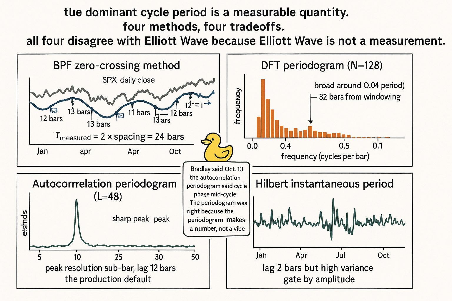
Comparison on SPX daily
Apply all four methods to SPX daily, 2020-2024. Compare period estimates, lag, and stability.
Four readings.
The BPF zero-crossing is the simplest but has visible resonance bias: the average estimate of 23.4 bars sits close to the BPF center period of 20, suggesting the BPF is pulling the measurement toward its passband.
The DFT periodogram with proper detrending produces a comparable mean estimate (26.1 bars) but with poorer resolution and substantially higher lag (32 bars vs the others). The lag makes it unsuitable for adaptive indicator tuning.
The autocorrelation periodogram is the best balance: 24.7-bar mean estimate, lowest standard deviation (3.1 bars), and acceptable lag (12 bars). The standard deviation is approximately one-third of the DFT's, indicating much more stable bar-to-bar estimates.
The Hilbert method has the lowest lag (2 bars) but the highest standard deviation (8.6 bars). The high variance reflects the phase-derivative noise. Used alone, the Hilbert estimate is too jittery for practical adaptive indicators. Combined with a smoother method (e.g., autocorrelation periodogram for the steady-state estimate and Hilbert for transition detection), it adds responsiveness without sacrificing stability.
The astrology contrast
Three cycle theories are widely circulated but produce no testable measurement.
Elliott Wave: claims the market moves in a five-wave impulse and three-wave correction structure with specific Fibonacci ratios between wave lengths. The "wave count" is determined by the analyst's visual interpretation of the chart and is not produced by any algorithm. Multiple wave counts can be drawn on the same data. When a prediction fails, the analyst revises the count post hoc. There is no falsifiable claim about the dominant cycle period that can be compared to the autocorrelation periodogram.
Gann theory: uses geometric angles (45 degrees, 1×1, 2×1, etc.) and time cycles derived from astronomical periods to predict turning points. The "law of vibration" is asserted as a master cycle. Cycle periods are claimed but not derived from the data; they are imposed from astronomical or numerological relationships. When applied to actual price data, Gann angles produce visually plausible levels that do not correspond to any spectral peak in the autocorrelation analysis.
Bradley turn dates: derived from planetary aspect calculations. The dates are precise (October 13, 2024, for example). The claim that turns occur on these dates is publicly testable. Studies that have tested it find no statistical significance beyond chance, but the dates continue to circulate in trading commentary because individual hits are memorable and individual misses are excused.
The structural failure mode of all three: they make claims about cycle structure that cannot be validated against the autocorrelation periodogram or any other measurable spectral quantity. They are not theories of market cycles; they are pattern recognition in the absence of measurement.
This article is not a debunking of all "cycle" claims. Markets do have measurable cycles (the autocorrelation periodogram on SPX has clear peaks in the 15-35-bar range). The claim is that the empirical cycle structure is the thing worth measuring, and the empirical methods give answers that disagree with the astrology methods.
What this changes in practice
Five operational shifts.
Default to the autocorrelation periodogram for dominant cycle estimation. The construction has the right balance of latency, precision, and robustness for production use. The Hilbert method serves as a low-latency complement when transition detection matters.
Feed the cycle estimate to all cycle-mode indicators. The article "Band-Pass Filters: The Most Underused Tool in Technical Analysis" used the cycle period as the BPF's center parameter. The article "Decyclers: Extracting Trend by Removing Cycle Energy" used it as the decycler's cutoff. The article "Automatic Gain Control for Trading Indicators" used it for the AGC window length. Each indicator becomes adaptive when fed the live estimate.
Report cycle estimates with confidence intervals. The autocorrelation periodogram's peak has a width that indicates confidence: a sharp peak means high confidence in the period estimate, a broad peak means low confidence. Strategies that consume the estimate condition their behavior on the confidence: only act when confidence is high, default to trend-mode logic when confidence is low.
Gate cycle-mode strategies by the periodogram peak quality. When no clear peak exists (the periodogram is approximately flat across the period range), the market is in trend mode and cycle-mode strategies should be disabled. The peak-vs-floor ratio of the periodogram is the gating metric.
Reject all "cycle" claims that do not produce a numerical period estimate. Elliott Wave, Gann, Bradley, lunar cycles, and similar frameworks claim cycle structure without specifying which spectral peak they reference. The rejection is operational, not philosophical: if a cycle framework cannot produce a number that the autocorrelation periodogram can confirm or refute, it cannot inform adaptive indicator tuning and cannot be backtested.
Decision matrix
| Use case | Recommended method | Reason |
|---|---|---|
| Production adaptive indicator tuning | Autocorrelation periodogram | Best balance of latency, precision, robustness |
| Real-time transition detection | Hilbert instantaneous + autocorr fallback | Hilbert speed, autocorr stability |
| Diagnostic spectrum visualization | DFT periodogram (with detrending) | Full spectrum view |
| Quick check / lightweight implementation | BPF zero-crossing (wide-band) | O(1) per bar |
| Multi-cycle decomposition | DFT or comb filter bank | Resolve multiple peaks |
| Cycle mode vs trend mode gate | Autocorrelation periodogram peak quality | Peak-to-floor ratio |
| Cross-instrument cycle comparison | Autocorrelation periodogram | Consistent definition across instruments |
| Backtesting cycle-period regime regimes | Autocorr periodogram at every bar | Reproducible numerical history |
Anti-patterns
Five mistakes that show up in cycle-based trading.
Anti-pattern 1: trading off Elliott Wave counts, Gann angles, Bradley turn dates, or any other cycle framework that does not produce a numerical period that can be validated against the autocorrelation periodogram. The frameworks are unfalsifiable, and the trading edge (if any) is indistinguishable from random pattern recognition.
Anti-pattern 2: assuming "the dominant cycle is 20 bars" as a constant. Real cycle periods drift over weeks and months. A static cycle assumption breaks adaptive indicators precisely when they are most needed (regime transitions).
Anti-pattern 3: using DFT without detrending on raw price data. The annual and semi-annual cycles dominate the spectrum and obscure the trading-relevant 15-35-bar peaks. The fix: HPF the input at the longest cycle of interest before the DFT.
Anti-pattern 4: trusting the Hilbert period estimate when the cycle amplitude is low. The phase derivative becomes noise-dominated during trend mode. Gate the Hilbert estimate by an amplitude threshold; use the autocorrelation periodogram as fallback when amplitude is low.
Anti-pattern 5: treating the cycle period estimate as a prediction. The estimate describes the current cycle structure based on past data. It does not predict when the next peak or trough will occur. Strategies that condition on "the next peak is N bars away" are extrapolating from a backward-looking estimate.
Visualizing the empirical cycle
KEY POINTS
- The dominant cycle period is a measurable quantity: the period T at which the autocorrelation function of the detrended series has its largest non-trivial peak. Computable, falsifiable, comparable across methods.
- Four established methods produce numerical estimates with known tradeoffs:
- BPF zero-crossing: simplest, O(1), 5-bar lag, sensitive to BPF resonance bias
- DFT periodogram: classical, 32-bar lag, coarse resolution, spectral dilation issues
- Autocorrelation periodogram: preferred default, 12-bar lag, fine resolution, robust
- Hilbert instantaneous: lowest 2-bar lag, high variance, requires amplitude gating
- The autocorrelation periodogram is the operational default. Best balance of latency, precision, and robustness.
- The Hilbert method is the complement for low-latency transition detection. Use both: autocorr for steady-state, Hilbert for change detection.
- On SPX 2020-2024: dominant cycle period estimates cluster around 24-26 bars with std deviations of 3-9 bars depending on method.
- Cycle estimates are not predictive. They describe current cycle structure based on past data. They do not extrapolate to when the next peak or trough will arrive.
- Cycle estimates feed adaptive indicators: BPF center period, decycler cutoff, AGC window length all update bar-by-bar from the live estimate.
- Gate cycle-mode strategies by the periodogram peak quality. When no clear peak exists, the market is in trend mode and cycle-mode logic should be disabled.
- Elliott Wave, Gann angles, Bradley turn dates, and similar frameworks make cycle claims that do not produce numerical period estimates testable against the autocorrelation periodogram. They are pattern recognition in the absence of measurement.
- Reject cycle frameworks that cannot specify which spectral peak they reference. The test is operational: if the framework cannot produce a number, it cannot inform adaptive indicators or backtests.
- Real market cycles are weak, time-varying, and often multiple. The empirical estimate is imperfect but the imperfection is itself a measurable property. The next article in this series ("Why Market Cycles Are Evanescent") expands on the persistence and stability properties.
- The astrology contrast is operational, not philosophical: if a cycle theory cannot disagree with the autocorrelation periodogram, it does not inform any trading decision the periodogram cannot inform more honestly.
References
- Statistically Sound Indicators for Financial Market Prediction - Timothy Masters (Amazon)
- Cycle Analytics for Traders - John Ehlers (Amazon)
- Hierarchical Endogenous Market-State Representation for Financial
- Why 42% of Turn-Level Findings in LLM Conversation Analysis May
- Price-Driven Multi-Agent LLMs for High-Frequency Trading - arXiv
- Multi-scale periodic analysis of financial indexes for quantitative
- Full article: Time-Series Predictability for Sector Investing
- Deep Autocorrelation Modeling for Time-Series Forecasting - arXiv
- Financial Signal Processing and Machine Learning | Wiley
- Determinism in Business Cycles: Kaldor-Kalecki's Model 80 Years