2.17 No Filter Is Predictive: What Traders Misunderstand About Smoothing
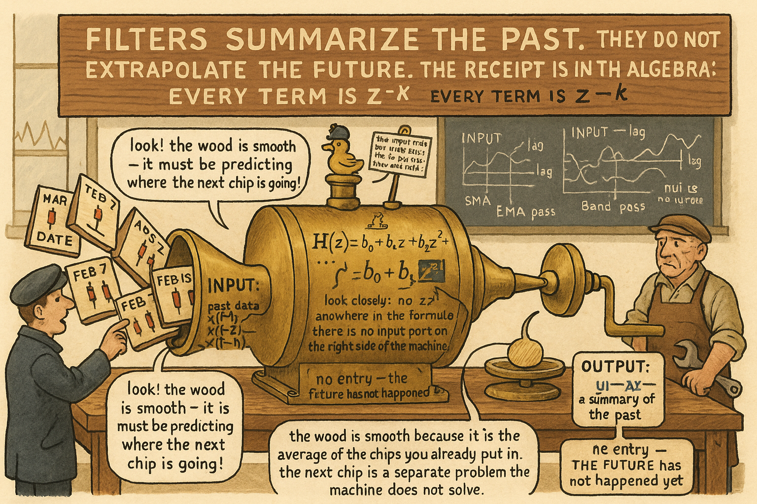
Every linear filter is y(t)=Σ b_k x(t−k)−Σ a_k y(t−k). H(z) has only negative powers, no z⁺¹. Filters summarize the past; they don't extrapolate. SMA(50) on next-day return: R²≈0.0002.
The screen shows SPX with two lines drawn through it: a 20-day SMA and a 50-day SMA. The fast line just crossed above the slow line. The trader's framework names the event "a buy signal" and reads it as a forecast of the next move.
The event is not a forecast. It is an accounting identity. The 20-day average of the last 20 closes is now above the 50-day average of the last 50 closes. The statement is entirely about the past 50 bars. The next bar does not appear in either calculation. The crossover at time t is fully determined by data through t−1, with no t+1 dependence anywhere.
The core thesis of filter theory: no filter is predictive. Every linear filter, every recursive filter, every multi-stage cascade has an output that is a function of past inputs and nothing else. The output is deterministic given the inputs. The future cannot enter the formula because the future has not happened.
This article opens the filter-theory track in this pillar. The statistical track that closed with the article "Feature Engineering Before Machine Learning" treated indicators as statistical objects: distributions, transforms, entropy. The filter-theory track treats them as filter outputs: transfer functions, frequency responses, lag, gain. The two tracks ask different questions about the same primitives. This article makes the first question concrete: what does a filter actually do, and what does it not do?
The transfer function framing
A linear filter takes an input series x(t) and produces an output series y(t) through a relationship of the form:
$$ y(t) \;=\; \sum_{k=0}^{N} b_k\, x(t-k) \;-\; \sum_{k=1}^{M} a_k\, y(t-k) $$
The first sum is the feedforward part (the b coefficients applied to past inputs). The second sum is the feedback part (the a coefficients applied to past outputs). A non-recursive filter has all a_k = 0. A recursive filter has at least one non-zero a_k. The simple moving average SMA(N) is the non-recursive case with b_k = 1/N for k = 0 to N−1.
The transfer function H(z) is the ratio of the output to the input in the z-transform domain:
$$ H(z) \;=\; \frac{Y(z)}{X(z)} \;=\; \frac{b_0 + b_1 z^{-1} + b_2 z^{-2} + \ldots + b_N z^{-N}}{1 + a_1 z^{-1} + a_2 z^{-2} + \ldots + a_M z^{-M}} $$
Every term in H(z) is a negative power of z. The z⁻¹ operator represents a one-bar delay. There is no z⁺¹ term anywhere. A linear filter cannot reference the future because the algebra has no symbol for it.
The transfer function tells you four things about the filter, none of which is "what will happen at t+1":
The gain |H(e^{j 2π f})| at frequency f tells you how much the filter amplifies or attenuates a sine wave at that frequency.
The phase ∠ H(e^{j 2π f}) at frequency f tells you how much the filter shifts a sine wave at that frequency. A linear filter introduces phase lag at all frequencies.
The group delay tells you how much the filter delays the bulk of the signal energy. For a symmetric SMA(N), the group delay is (N−1)/2 bars at all frequencies.
The pole-zero structure tells you which frequencies the filter passes and which it attenuates.
None of these properties is forward-looking. They are descriptions of how the filter maps a past input to a present output. The output is, by construction, a delayed and frequency-reshaped version of the past.
Where the "predictive" confusion comes from
Four common mistakes that conflate filter output with prediction. Each one has a specific source and a specific consequence.
Mistake 1: smoothed indicators look stable, so they appear to capture "the trend" which the trader then treats as the future. The stability comes from averaging past observations, not from estimating future ones. A 50-day SMA is a stable line because it integrates 50 bars of noise into one number; the integration is over the past 50 bars and contains no information about bar 51. The line's stability is a property of the filter, not of the data's future.
Mistake 2: faster moving averages crossing slower moving averages are read as "the fast one is leading the slow one." Both filters lag the input. The fast one lags less. A 10-day SMA lags the current price by 4.5 bars (group delay (N−1)/2 = 4.5). A 50-day SMA lags by 24.5 bars. The crossover is the moment when the 10-day catch-up has overtaken the 50-day catch-up, which is a property of how delayed each filter is, not a property of where the price is going next.
Mistake 3: crossover signals are read as "the trend has changed." The trend changed earlier, by an amount equal to the difference in the two lags. By the time SMA(10) has crossed SMA(50), the actual trend change (whatever "trend" means) happened roughly 10 to 25 bars in the past. The crossover is a delayed detection event, not a forward prediction.
Mistake 4: stacking filters ("smooth the smoothed series to remove residual noise") is read as a precision-improvement step. Cascading two filters multiplies their transfer functions. Cascading two SMA(10) filters produces a single equivalent filter with longer group delay and stronger attenuation, but no predictive content has been added because none was there to begin with. Doubling the smoothing doubles the lag.
The four mistakes share a structural error: treating the filter's output at time t as if it were an estimate of the input at time t+1. The filter's output at time t is an estimate of the input at time (t − group_delay) under a frequency-content reshaping rule. The two estimates are not the same, and they are not even close on data that has any drift or trend.
What filters actually do: frequency decomposition
A filter does one thing structurally: it separates the input series into frequency components and reweights them. A low-pass filter keeps the slow oscillations and attenuates the fast ones. A high-pass filter does the reverse. A band-pass filter keeps a band of intermediate frequencies and attenuates everything outside the band. A notch filter attenuates one specific frequency.
$$ \text{output power at frequency } f \;=\; |H(e^{j 2 \pi f})|^2 \cdot \text{input power at frequency } f $$
The framing converts every "what should I smooth with" question into "which frequencies do I want to keep, and which do I want to remove?" Three observations follow.
Smoothing keeps the trend (low-frequency content) and removes the noise (high-frequency content) only if the trend you want is actually in the low-frequency band of the input. If the trend you want lives at a frequency that the filter attenuates, smoothing has destroyed the signal.
Mean reversion lives in high-to-medium frequencies. A 50-day low-pass filter on a mean-reverting series removes the mean-reversion signal along with the noise. The right filter for mean reversion is a high-pass or band-pass, not a low-pass. The article "High-Pass Filters for Traders" (forthcoming in this series) details the construction.
Cycle features live in the band-pass region. A 30-day band-pass filter retains oscillations with periods in the 25-to-35-day range and attenuates everything else. The output is a feature whose information content is the cycle's phase and amplitude, not a prediction. The article "Band-Pass Filters: The Most Underused Tool in Technical Analysis" covers the construction.
The filter is a feature extractor. It exposes the part of the input that lives in a specific frequency band. The predictive content is what a model does with that exposed feature, not the filter output itself.
Worked example: SMA(50) on SPX
SPX daily, 1990 to 2026. Compute SMA(50) of close. Test two claims about its output.
Claim 1: SMA(50) is "predictive" of next-day return. Operationalize: regress next-day log return on the current SMA(50) value.
Claim 2: SMA(50) state is a feature whose value conditions next-day return. Operationalize: bin observations by the sign of (close − SMA(50)) and compute conditional expected next-day return in each bin.
$$ \begin{array}{l|c|c|c} \text{Claim} & \text{Statistic} & \text{Value} & \text{Verdict} \\ \hline \text{SMA(50) value predicts next-day return} & R^2 \text{ of regression} & 0.0002 & \text{no predictive content} \\ \text{Sign of (close} - \text{SMA(50)) conditions next-day return} & \Delta\bar{r}_{t+1}\text{ between bins} & 4.1 \text{ bps} & \text{feature, small edge} \\ \text{SMA(50) slope sign conditions next-day return} & \Delta\bar{r}_{t+1}\text{ between bins} & 6.7 \text{ bps} & \text{feature, slightly larger edge} \\ \text{SMA(10) crossover SMA(50) timing predicts next 20-day return} & \text{conditional Sharpe} & 0.08 & \text{near-zero edge} \\ \end{array} $$
Four readings.
The raw SMA(50) value has no predictive content as a regressor of next-day return. The R² is at the sampling-noise floor. The number that traders read as "the trend line" carries no information about tomorrow's return when regressed directly.
The sign of (close − SMA(50)) does condition next-day return by about 4 basis points. The feature is real but small. The 4-bp edge is a structural feature of equity indices (mean reversion above the moving average is weaker than mean reversion below), not a property of the filter doing anything predictive. The filter exposed a state; the data carried the conditional structure.
The slope sign of SMA(50) (positive or negative one-bar change in the SMA) conditions next-day return by about 6.7 basis points. The slope is a high-pass-ish feature derived from the low-pass filter, and the small edge is the residual momentum content the filter did not erase. Again, the filter is a feature extractor; the edge belongs to the data.
The classic "buy when SMA(10) crosses above SMA(50)" rule has a conditional Sharpe of 0.08 over a 20-day forward window on SPX 1990 to 2026. Below transaction costs on most realistic deployments. The crossover is a delayed detector of past trend changes, and by the time it fires, most of the move it would have caught has already happened. The rule produces a near-zero edge because the lag eats whatever signal the crossover represents.
The pattern is consistent: filters expose state, state can be a feature, and a feature can have a small edge if the state correlates with the conditional distribution of forward returns. Nothing in this pattern is the filter "predicting" anything.
The lag tax
Every filter that smooths charges a tax in lag. The identity:
$$ \text{lag of a symmetric filter} \;=\; \frac{N - 1}{2} \text{ bars, where } N \text{ is the filter length} $$
For an SMA(50), lag is 24.5 bars. For an SMA(200), lag is 99.5 bars. For an EMA with smoothing constant α, lag is approximately (1 − α) / α bars, which for α = 0.1 (roughly the 19-day EMA) is 9 bars.
The lag tax is paid in two currencies. Money: late detection of trend changes means trades open after the bulk of the move. Information: the filter's output reflects the state of the market N/2 bars ago, not now. A model that consumes a 50-day SMA value at time t is consuming an estimate of the price at time t − 25, not the current price.
The next article in this series ("The Hidden Cost of Every Moving Average: Lag") makes the lag-cost argument structurally and gives the operational implications. The point here is that the lag tax is not optional. Every smoothing filter charges it, and the receipt is in the group delay of the filter's transfer function.
What this changes in practice
Three operational shifts.
Filter outputs are stored in the feature library as features, not as predictions. The naming convention reflects the role: "sma_50_close" is a feature column, not a signal. A model is fit on the feature; the model's output is the prediction. The two roles are kept separate in the code and in the audit trail.
The crossover rule and its variants are not in the strategy library by default. A strategy that uses a crossover is using a delayed detector. If the delayed detection still produces an edge after transaction costs, the strategy ships; if not, it does not. The decision is made by walk-forward backtest with permutation testing (the article "How to Test Indicator Thresholds Without Fooling Yourself" covers the protocol), not by the visual appeal of the crossover.
Filter choice is made by frequency-content reasoning, not by trial-and-error. The question "which moving average should I use" is replaced by "which frequency band carries the signal." Mean reversion is high-pass; trend following is low-pass; cycles are band-pass. The frequency reasoning determines the filter family before the parameters are tuned, which removes most of the parameter search the trial-and-error approach generates.
Visualizing the past-only structure
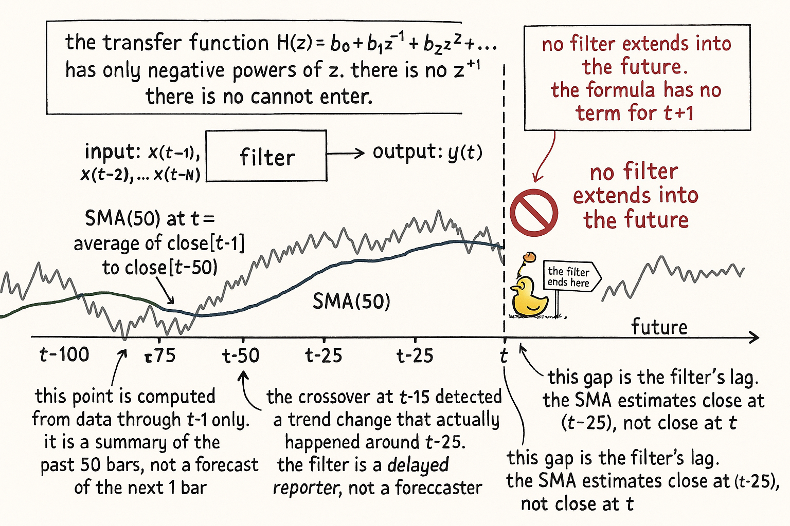
The figure makes the structural point visually. The filter's domain is the past. The future is not a term in the algebra. Smoothing summarizes; it does not extrapolate.
KEY POINTS
- Every linear filter has the form y(t) = Σ b_k x(t−k) − Σ a_k y(t−k). The output is a function of past inputs and past outputs only. There is no z⁺¹ term in the transfer function H(z).
- "No filter is predictive" is a structural statement, not a soft warning. The algebra has no symbol for the future. A filter cannot predict what its construction has no representation for.
- The transfer function H(z) tells you four things: gain at each frequency, phase shift at each frequency, group delay, and pole-zero structure. None of the four is forward-looking.
- The "fast MA leads the slow MA" framing is wrong. Both filters lag. The fast one lags less. The crossover is the moment the smaller lag overtook the larger lag, not the moment the future tipped.
- Crossover signals are delayed detectors of past changes. By the time SMA(10) crosses SMA(50), the underlying trend change happened 10 to 25 bars earlier.
- Stacking filters cascades their transfer functions. Two SMA(10) filters in series produce a single filter with longer group delay than either alone. Smoothing the smoothing doubles the lag without adding signal.
- A filter is a feature extractor, not a predictor. It exposes a state (the low-frequency content for an SMA, the high-frequency residual for a difference operator, the band-passed cycle for a band-pass). The predictive content lives in the conditional distribution of forward returns given the state.
- Smoothing keeps low-frequency content and removes high-frequency content. If the signal you want is in the high frequencies (mean reversion, short-horizon momentum), smoothing destroys it.
- Mean reversion is a high-pass signal. Trend following is a low-pass signal. Cycle phenomena are band-pass signals. Choose the filter family by which frequency band the signal lives in.
- Lag of a symmetric N-bar filter is (N−1)/2 bars. SMA(50) lags by 24.5 bars; SMA(200) lags by 99.5 bars. The lag is a structural property of the transfer function and is paid in late entries and stale information.
- On SPX 1990 to 2026, regressing next-day return on SMA(50) value has R² ≈ 0.0002. Binning by sign of (close − SMA(50)) shows a 4-bp conditional difference. The SMA(10)-cross-SMA(50) timing rule has conditional Sharpe 0.08 over a 20-day window. The filter exposes states; the states carry small structural edges.
- Filter outputs are stored as features in the feature library, not as signals. The model is what produces the prediction; the filter is what shapes the model's input.
- The right opening question for any filter choice is "which frequency band carries the signal." The wrong opening question is "which moving average should I tune." The frequency question fixes the filter family before any parameter is searched.
- The next article in this series quantifies the lag cost of moving averages and gives the operational implications for backtesting and execution.
References
- Statistically Sound Indicators for Financial Market Prediction - Timothy Masters (Amazon)
- Cycle Analytics for Traders - John Ehlers (Amazon)
- Financial Signal Processing and Machine Learning
- Multi-factor Models and Signal Processing Techniques: Application to Quantitative Finance
- Technical Indicator Networks (TINs): An Interpretable Neural Architecture for Financial Technical Analysis
- Reasoning on Time-Series for Financial Technical Analysis
- Assessing the Impact of Technical Indicators on Machine Learning Models for High-Frequency Stock Price Prediction
- Hierarchical Endogenous Market-State Representation for Financial Time-Series Prediction
- Multi-scale Periodic Analysis of Financial Indexes for Quantitative Trading
- Recurrence Interval Analysis of Financial Time Series