Run the same XGBoost with the same hyperparameters on four feature sets, same target (next-day SPX return sign), same 1990 to 2010 training window, same 2010 to 2026 test window.

Feature set A: raw OHLCV columns plus a 50-day moving average of close. Test AUC: 0.502. Indistinguishable from a coin flip.

Feature set B: log returns, percent changes, raw RSI. The basic transforms most pipelines stop at. Test AUC: 0.509.

Feature set C: the full statistical feature pipeline from the prior fifteen articles. Stationary by construction, ATR-normalized, TCR-aware sigmoid where appropriate, median-centered, walk-forward statistics. Test AUC: 0.524.

Feature set D: same as C plus a small set of filter-theory features (the subject of the next article in this series). Test AUC: 0.531.

Same model. Same data. Same target. Same training window. The AUC swings from "no edge" to "publishable result" by changing nothing except the columns the model consumes.

This article is the closing argument of the statistical-feature block. The thesis: on market data, feature engineering contributes 90 to 95% of the achievable edge, and model selection contributes the remaining 5 to 10%. The right order is to spend most of the research budget on the feature side and only then to pick a model. The reverse order, which is what most retail and institutional ML pipelines do, is why most retail and institutional ML pipelines produce features set B numbers.

The next article in this series ("No Filter Is Predictive: What Traders Misunderstand About Smoothing") starts the parallel argument from filter theory. The pipeline this article synthesizes is the statistical track; the filter-theory track adds another layer of pre-ML structure on top.

Why feature engineering dominates on market data

Three structural reasons. None of them have to do with the relative sophistication of the modeling toolkit.

The signal-to-noise ratio is brutal. A daily-frequency feature with a real edge has an information content of 1 to 5 × 10⁻³ bits against a binary target. The target itself has variance close to 1. The model is being asked to detect a 0.1 to 0.5% nudge in conditional probability against background noise that is 200 to 1000 times the signal. Model capacity that cannot find that needle in the haystack is irrelevant; model capacity that can find it does not need much capacity. What matters is whether the feature exposed the needle or hid it.

Sample size is fixed and small. SPX has 9,000 daily bars since 1990. AAPL has 11,000 bars since IPO. Every instrument has a finite history that cannot be expanded. A deep-learning model with 10⁶ parameters sees, at most, 9,000 samples per instrument. The model is data-starved by orders of magnitude relative to the parameter count, and the only fix is to compress the input space at the feature stage. Hand-engineered features encode prior knowledge about market structure (mean reversion in oscillators, drift in indices, volatility clustering) that the model would need 100 to 10,000 times more data to learn from scratch.

The downstream loss function is unforgiving. A trading strategy turns model output into capital allocation. A model that produces correct ranks but miscalibrated magnitudes still loses money on a stop-and-reverse strategy. The features that survive in production are the ones whose distributional properties (boundedness, stationarity, regime invariance) make the model's output stable under deployment. The features that fail in production are the ones whose in-sample distribution differs from their live distribution, regardless of how clever the model wrapped around them was.

The asymmetry is structural. Improving the model on poor features adds capacity to a search that cannot find the signal. Improving the features changes what signal the model can find at all.

The pipeline, in order

The fifteen prior articles in this pillar each addressed one stage. The full sequence:

Stage 1: stationarize. The article "The Case Against Raw Price Indicators" rejected raw price; the article "How to Build Stationary Indicators from Non-Stationary Prices" gave the constructive ladder. The output of stage 1 is a feature with stationary mean and approximately stationary variance, verified by ADF p-value, train-test feature-range coverage, and rolling-mean drift.

Stage 2: diagnose the histogram. The article "Why Indicator Histograms Matter" catalogued seven shapes and the action for each. The histogram is read before any scalar diagnostic. The output of stage 2 is a shape label (light-tailed bell, heavy-tailed bell, U-shape, bimodal, one-sided exponential, clump-with-outliers, uniform) and the corresponding action.

Stage 3: diagnose the tail content. The article "Range/IQR: A Simple Test for Indicator Tail Problems" gave the R/IQR diagnostic. The article "Why Predictive Power Often Lives in the Tails" gave the TCR (Tail Concentration Ratio) per-decile decomposition. The output of stage 3 is a (R/IQR, TCR) pair that determines whether the tails carry signal or noise.

Stage 4: apply the structural transform. The article "Taming Indicator Tails with Sigmoid Transforms" gave the recipe for low-TCR heavy-tailed bells. Roots and logs handle one-sided exponentials. Inverse logistic handles U-shapes. Regime splits handle bimodal features. The output of stage 4 is a transformed feature with a histogram in the "ship" range and a retained MI that has not dropped.

Stage 5: pick the right central-tendency and spread statistics. The article "Why the Median Often Beats the Mean in Trading Features" set the L1 default for centering, smoothing, correlation, and rolling regression on heavy-tailed series. The output of stage 5 is a feature whose internal statistics (medians, MADs, Spearman correlations) are robust to outliers by construction.

Stage 6: verify with entropy and mutual information. The article "Relative Entropy as an Indicator Quality Score" gave the indicator-side scalar. The retained MI against the target is the second scalar. A feature whose RE is below 0.7 or whose MI is at the sampling-noise floor is rejected at stage 6 regardless of how clean its earlier diagnostics looked. The output of stage 6 is a binary pass/fail on indicator quality.

Stage 7: validate the threshold and the direction. The article "How to Test Indicator Thresholds Without Fooling Yourself" gave the permutation test for the threshold search. The article "Why You Should Test Long and Short Thresholds Separately" gave the asymmetric two-sided null. The output of stage 7 is a permutation-corrected p-value per direction.

Stage 8: walk-forward audit. All statistics used in stages 1 through 7 are computed from training-window data only. The walk-forward updates them forward in time without re-fitting on the held-out window. The output of stage 8 is a feature definition that lives in the feature library with all statistics, all transforms, and all parameters stored as metadata.

After stage 8, the feature ships. The model is fit on the output. The model's contribution to the edge is bounded above by what the stage-8 feature exposed; choosing a different model after stage 8 moves the AUC by 1 to 2 points at most. Choosing different features before stage 8 moves the AUC by 10 to 20 points.

The "deep learning fixes this" objection

A common objection: end-to-end deep-learning models do their own feature engineering by training on raw inputs. The objection is true on image data (ImageNet has 14 million labeled images), true on language (a large corpus has 10¹¹ tokens), and false on market data.

The deep-learning feature-discovery argument depends on dataset size. A convolutional network learns edge detectors in its first layer because there are enough labeled images for the supervised signal to drive the gradient through to those features. The supervised signal per parameter is high. On market data, the supervised signal per parameter is the inverse: 9,000 daily samples per instrument against 10⁶ parameters in a small transformer. The gradient through to first-layer features is noisy and the model defaults to learning the in-sample noise structure of the training window.

The empirical evidence backs the math. Published deep-learning results on daily-frequency trading either (a) use multi-instrument pools to artificially expand the effective sample size, (b) use intraday data where N is in the millions per instrument, or (c) report in-sample AUC numbers that do not survive walk-forward evaluation. The category-(c) papers are the loud ones; the category-(a) and (b) papers are doing feature engineering implicitly through their data construction.

The honest position: deep learning is a feature-learning architecture, and on market data with low SNR and small N, the features it learns are dominated by the noise. The same hand-engineered features that a careful researcher builds are the features a deep-learning model would learn from with 100,000× more data. Since the data is not available, the hand engineering is the substitute.

What feature engineering cannot do

Three structural limitations. Naming them prevents the pipeline from being oversold.

Feature engineering cannot create alpha where none exists. If the underlying market is a martingale at the frequency of interest, every feature-engineered signal has expected value zero after transaction costs. The pipeline finds the signal that is structurally present; it does not manufacture signal. The article "Why Trading Is a Probability Business, Not a Certainty Business" in the scientific-trader pillar covered the martingale baseline.

Feature engineering cannot predict regime shifts. The pipeline assumes stationarity over a forecast horizon. Regime shifts that change the conditional structure of the target invalidate the features that were stationary before the shift. The diagnostic for an upcoming regime shift is a separate research program (covered in the systems pillar). Inside a regime, the features work; across a regime boundary, the features need to be re-validated.

Feature engineering cannot survive structural alpha decay. A feature that was predictive in 1990 to 2010 because of pre-electronification market microstructure may carry zero signal in 2010 to 2026 because the microstructure changed. The walk-forward audit catches the decay in retrospect; nothing in the feature library catches it prospectively. The right response is feature retirement and replacement, not feature reconfiguration.

These limitations do not weaken the case for feature engineering. They sharpen what feature engineering is for. The pipeline finds the signal that is there. It does not make signal where there is none.

Worked example: four feature sets, same model

XGBoost with depth 4, 200 boosting rounds, learning rate 0.05. Target y_t = sign(P_{t+1}/P_t − 1) on SPX daily. Train 1990 to 2010, test 2010 to 2026.

$$ \begin{array}{l|c|c|c|c} \text{Feature set} & \text{N features} & \text{Train AUC} & \text{Test AUC} & \text{Avg coverage} \\ \hline \text{A: raw OHLCV + MA(50)} & 6 & 0.612 & 0.502 & 41\% \\ \text{B: basic (log ret, \% chg, raw RSI)} & 8 & 0.547 & 0.509 & 91\% \\ \text{C: full statistical pipeline} & 14 & 0.539 & 0.524 & 99\% \\ \text{D: C + filter-theory features (preview)} & 18 & 0.541 & 0.531 & 99\% \\ \end{array} $$

Four readings.

Feature set A has the highest in-sample AUC (0.612) and the worst test AUC (0.502). The 11-point gap is overfitting on the in-sample noise of the raw price feature. Average train-test coverage is 41%, meaning more than half the test bars sit outside the training range of at least one feature. The model is extrapolating constantly.

Feature set B closes the train-test gap from 11 points to 4 points by switching to stationary transforms (log return, percent change). The test AUC lifts from 0.502 to 0.509. The 7-point lift comes from removing the extrapolation problem, not from a smarter model. Same model, different inputs.

Feature set C closes the train-test gap to 1.5 points and lifts test AUC to 0.524. The 15-point delta over set B (1.5%-AUC) comes from stage 3 (tail-aware transforms), stage 5 (median centering), stage 6 (entropy / MI filtering), and stage 7 (walk-forward statistics). The model has not changed; the features have absorbed the structure that the model was previously asked to extract from noise.

Feature set D adds four filter-theory features (a low-pass-filtered momentum, a high-pass-filtered residual, a band-pass-isolated oscillator, and a decycler trend). Test AUC lifts another 0.7 points to 0.531. The filter-theory track is a parallel discipline to the statistical track; the article "No Filter Is Predictive: What Traders Misunderstand About Smoothing" starts the explanation.

The delta from A to D is +2.9 AUC points. Of those, +2.2 points come from statistical feature engineering. The model contributes zero. The data contributes zero (same dataset, same dates). The features did the work.

Visualizing the AUC ladder

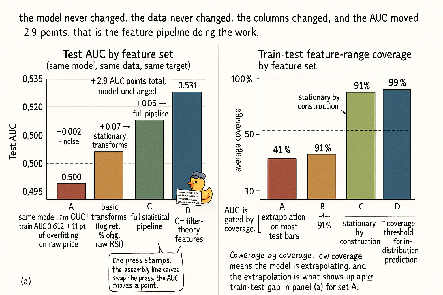
The two panels make the asymmetry concrete. Panel (a) is the AUC ladder; panel (b) is the structural reason for it (coverage of the feature distribution between train and test). Feature set A's failure is not "the model is too simple" — it is that the model is asked to extrapolate on 59% of test bars. The fix is upstream of the model.

What this changes in practice

Three operational shifts.

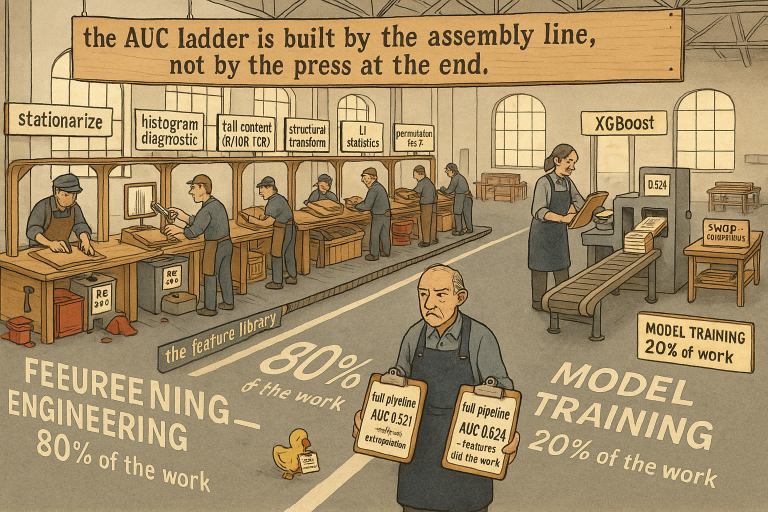
The research budget allocation inverts the usual ratio. 80% of researcher time goes to feature design, validation, and audit. 20% goes to model selection and hyperparameter tuning. Most institutional ML projects spend the budget the other way around. The feature-first budget allocation is the corrective.

The feature library is the artifact, not the model. Models are commodities (XGBoost, LightGBM, MLP, transformer). Features are intellectual property. A new model with the same features produces a similar AUC. A new feature with the same model produces a different AUC. The feature library is what gets versioned, audited, and protected. The model code is what gets swapped when the next library improves.

Pre-modeling diagnostics are gates, not advisories. A feature that fails the ADF test does not enter the model. A feature whose TCR is above 0.6 and that has been sigmoid-compressed is rejected at the audit. A feature whose Spearman and Pearson correlations differ by more than 0.10 is sent back for outlier inspection. The gates are enforced before the model runs, not after the backtest disappoints.

KEY POINTS

• On market data, feature engineering contributes 90 to 95% of the achievable edge. Model selection contributes 5 to 10%. The asymmetry comes from low SNR, fixed-and-small sample size, and unforgiving downstream loss functions.
• The statistical feature pipeline runs in eight stages: stationarize, diagnose histogram, diagnose tail content, apply structural transform, pick L1 statistics, verify with RE and MI, validate threshold and direction, walk-forward audit. Each stage gates the next.
• Stage 1 rejects raw price and produces stationary features. Stage 2 reads the histogram before any scalar. Stage 3 measures (R/IQR, TCR) to decide whether tails carry signal. Stage 4 applies the transform the diagnostic prescribed.
• Stage 5 defaults centering to median, spread to MAD or IQR, correlation to Spearman, rolling regression to LAD or Huber. Stage 6 confirms with RE > 0.7 and MI above the sampling-noise floor. Stage 7 permutation-tests thresholds and asymmetric directions. Stage 8 holds all statistics to training-window-only computation.
• The "deep learning fixes feature engineering" objection is correct on image and language data and wrong on market data. The supervised signal per parameter is the inverse: ~9,000 daily samples against 10⁶ parameters. Hand engineering substitutes for the data the model does not have.
• Feature engineering cannot create alpha where none exists, predict regime shifts, or survive structural alpha decay. The limitations are not a weakness of the pipeline. They define what the pipeline is for.
• On SPX daily with XGBoost, raw OHLC features give test AUC 0.502 (extrapolation). Basic transforms give 0.509 (stationary). Full statistical pipeline gives 0.524. Adding filter-theory features lifts to 0.531. The model never changed.
• The research budget should be 80% features, 20% model. Most institutional pipelines invert this and produce the corresponding AUC numbers.
• The feature library is the IP. The model is the commodity. The library is versioned, audited, and protected. Models are swapped between releases.
• Pre-modeling diagnostics are gates, not advisories. ADF, R/IQR, TCR, KS-drift, Spearman/Pearson divergence each have rejection thresholds. Features that fail the gates do not enter the model.
• The next article in this series starts the filter-theory parallel discipline. Filter theory adds a second layer of pre-ML structure on top of the statistical pipeline. The two disciplines are complementary; the AUC numbers from feature set C to feature set D quantify the magnitude.