2.13 Why Indicator Histograms Matter
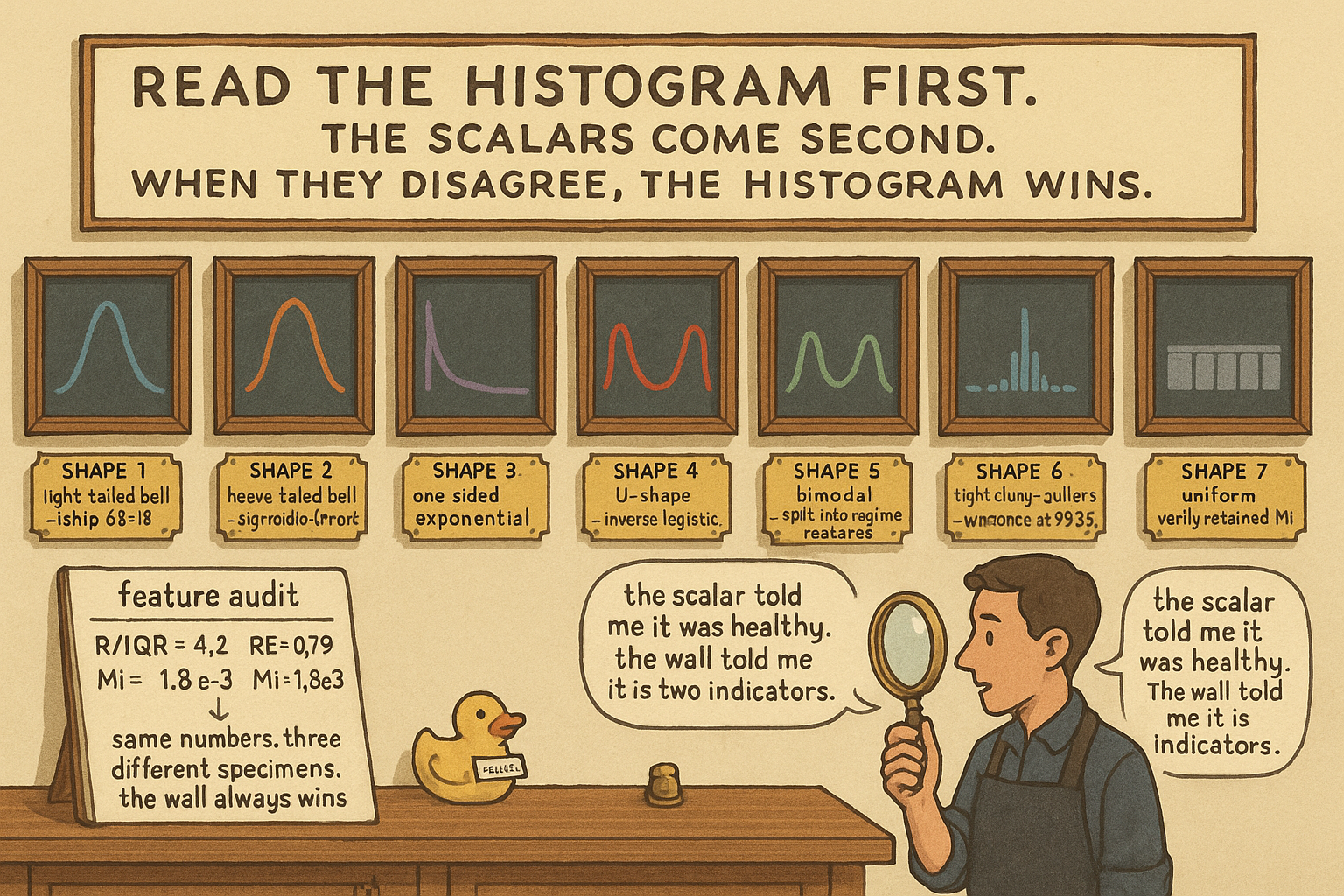
The histogram is the primary diagnostic. Scalars (R/IQR, RE, MI, TCR) confuse shapes needing different fixes. Identical scalars hide light-tail, heavy-tail, or bimodal — only bimodal needs a split.
You log three indicators in your feature library. All three have R/IQR = 4.2. All three have relative entropy = 0.79. All three have mutual information against next-day return sign of 1.8 × 10⁻³ bits. Three identical readings on the three scalar diagnostics.
The histograms tell three different stories.
The first histogram is a clean bell shape with light tails. Ship it.
The second histogram is a tight spike at zero with two thin wings reaching out to the diagnostic-allowed edges. Most of the mass lives in 5% of the range. The scalars say it is fine. The model trained on it will spend all its capacity on the central 5%, see a flat surface across the rest, and miss the predictive content that the thin wings carry.
The third histogram is bimodal: two equal humps at opposite ends with a valley in the middle. The scalars say it is fine. The indicator is mixing two market regimes whose conditional distributions of forward return are opposite, and the bimodality is the signal that the indicator should be split into two regime-conditional features.
This article is about the histogram as the primary visual diagnostic for indicator design. The summary scalars (R/IQR from the article "Range/IQR: A Simple Test for Indicator Tail Problems", relative entropy from "Relative Entropy as an Indicator Quality Score", TCR from "Why Predictive Power Often Lives in the Tails") are derived from the histogram. They compress it into one number each, and the compression loses information about shape that the scalars cannot represent. You read the histogram first. The scalars confirm what the histogram already said.
The constructive answer for one specific histogram shape (heavy-tailed bell) is the subject of the next article in this series ("Taming Indicator Tails with Sigmoid Transforms"). This article is the catalog of shapes and the decision matrix that follows from each one.
The seven shapes you will see
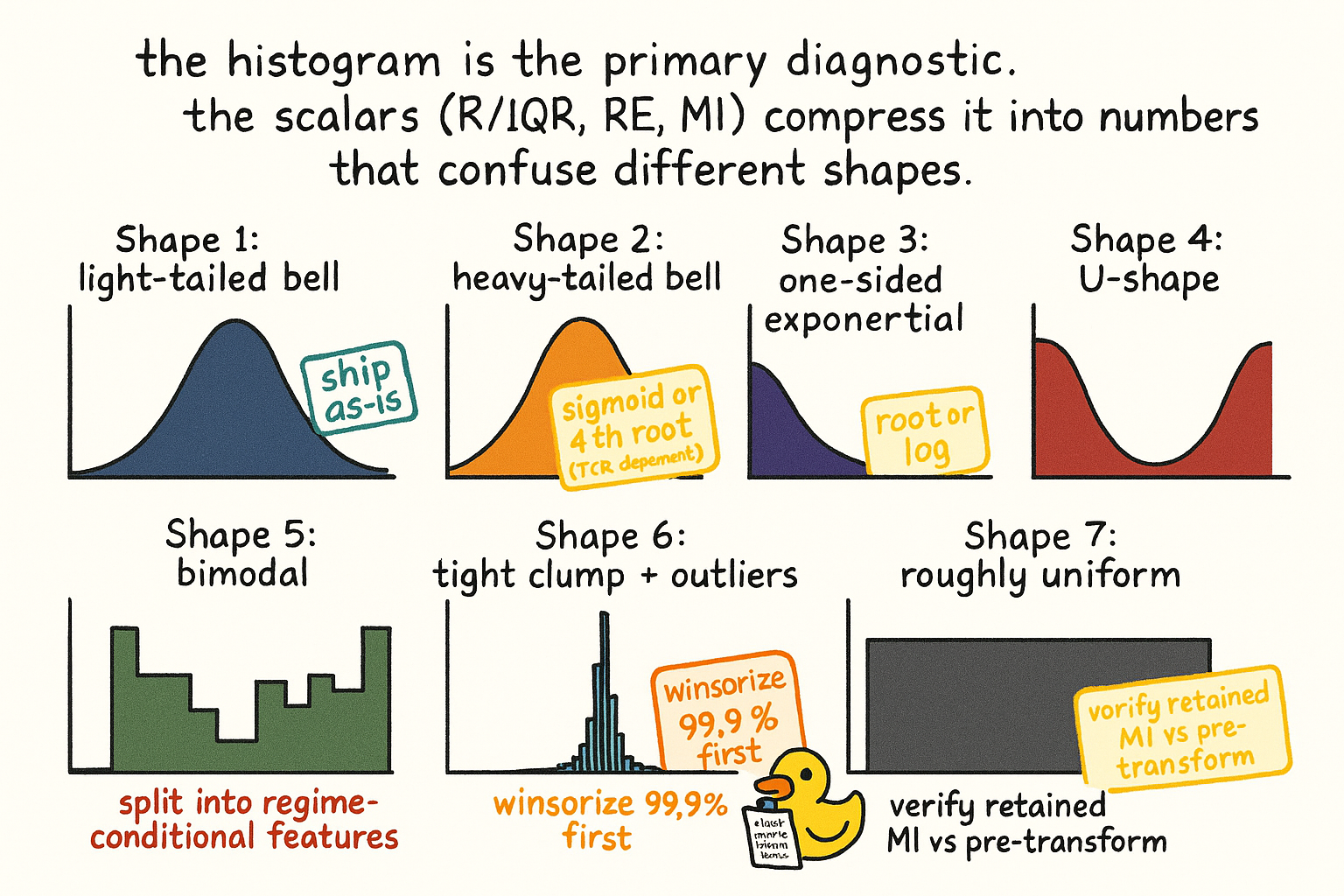
Most real indicators land in one of seven distributional shapes. Each shape has a structural cause, a structural consequence for the model, and a specific corrective action.
Shape 1: light-tailed bell. Roughly symmetric, single mode, tails that decay smoothly. The healthy default. RSI(14), 14-day stochastic K, Williams %R, and most ATR-normalized momenta on liquid instruments produce this shape. R/IQR is 2 to 4, relative entropy is 0.7 to 0.9, no transform required. Ship as-is.
Shape 2: heavy-tailed bell. Symmetric around a central mode, but the tails decay slowly and a small number of extreme observations sit far from the bulk. R/IQR is 6 to 15, relative entropy drops to 0.5 to 0.7 because most observations clump in the center. Same-bar OHLC differences before normalization, volume-based indicators, and most price-change indicators on stressed instruments produce this shape. The decision depends on tail-concentration: high TCR features keep their tails, low TCR features get a sigmoid. The article "Taming Indicator Tails with Sigmoid Transforms" gives the construction.
Shape 3: one-sided exponential decay. Mode at one edge of the range (usually zero), monotonic decay toward the other edge, no mass on the negative side. Volume, traded notional, absolute return, realized variance, and unsigned momentum produce this shape. R/IQR is high but irrelevant because the distribution is one-sided; relative entropy is low because most observations live near zero. The fix is a root (square root for mild, fourth root for moderate) or a log transform. Sigmoid does not help because the distribution is not centered.
Shape 4: U-shape. Modes at both edges, valley in the middle. RSI(2), short-lookback stochastic, and most divergence indicators on choppy markets produce this shape. R/IQR is low (the distribution is bounded), relative entropy is low (mass concentrated at edges). The shape is informative on its own (extreme readings are more common than central readings) but breaks linear regression and any model that assumes monotonic input-output relationships. The fix: inverse logistic transform, which maps the U-shape back to a bell. The article "How to Build Stationary Indicators from Non-Stationary Prices" mentioned the inverse logistic in passing; the operational rule is "U-shape → inverse logistic, no exceptions."
Shape 5: bimodal with separation. Two distinct humps, deep valley between them, similar mass in each hump. The indicator is mixing two market regimes whose distributions are different enough that the indicator cannot represent them as one feature. Cross-sectional features computed across mixed universes (equities + crypto) produce this shape. Half-life-based mean-reversion indicators on instruments that transition between trending and ranging produce this shape. The fix is not a transform; it is to split the indicator into two regime-conditional features and let the model condition on the regime as a separate input. The article on regime conditioning (forthcoming in the systems pillar) covers the split mechanics.
Shape 6: tight central clump with empty tails. Most observations in a narrow band (often 5 to 10% of the apparent range), a few isolated extreme values far out in the tails. R/IQR is high (the extremes inflate the range), relative entropy is low (the clump dominates the bin probabilities). The structural cause is usually a few outliers — data errors, splits not adjusted, a single Black Swan day — sitting in a feature otherwise well-behaved. The fix is winsorization at 99.5% or 99.9% before any other transform. The article "Range/IQR: A Simple Test for Indicator Tail Problems" covered the diagnostic; the histogram shows whether the offending observations are a continuous tail (real signal) or a few isolated points (data errors).
Shape 7: roughly uniform. Equal probability across the range. R/IQR is 1.5 to 2, relative entropy is above 0.95. The shape models prefer in principle. Almost never observed in raw indicators; usually appears only after an aggressive transform (rank, percentile, or histogram equalization). Uniform shape suggests the transform may have discarded magnitude information; check the retained MI against the un-transformed version to confirm the transform did not destroy signal.
What the scalars miss
Three diagnostics commonly used (R/IQR, relative entropy, MI) reduce the histogram to a number. The histogram contains shape information the number does not.
R/IQR confuses one isolated outlier with a heavy continuous tail. R/IQR = 12 from a feature with a clean bell shape and one Black Monday observation is a different problem from R/IQR = 12 from a feature with a continuously fattened tail. The first is fixed by winsorization at 99.9%. The second needs a sigmoid or fourth-root. The scalar does not distinguish them; the histogram does at a glance.
Relative entropy confuses a bimodal distribution with a uniform distribution at the same bin count. Two equal humps with a valley in between and a uniform distribution can produce identical relative entropy values when binned coarsely. The histogram shows the difference immediately; the entropy number reports them as identical-quality indicators.
Mutual information confuses a feature with signal in the tails and a feature with signal in the body. Same MI = 1.8 × 10⁻³ from a TCR = 0.78 feature (signal lives in the tail deciles) and from a TCR = 0.22 feature (signal lives in the body) are two different operational problems. The first needs the tails preserved; the second tolerates a sigmoid. The histogram, plotted alongside the per-decile MI bar chart from the article "Why Predictive Power Often Lives in the Tails", shows the difference.
Read the histogram first. Run the scalars second. When the scalars disagree with the histogram, the histogram wins.
Bin count and binning rules
The number of bins matters because shape diagnostics depend on resolution.
Too few bins (B = 5 to 10) smooth out the modes. A U-shape with B = 6 looks like an inverted bell. A bimodal distribution with B = 8 looks like a wide unimodal distribution. The cure is more bins.
Too many bins (B > N / 10 for N observations) introduce empty bins and sampling noise. A U-shape with B = 100 on N = 500 observations shows a jagged histogram where every other bin is empty, and the eye reads the noise rather than the shape. The cure is fewer bins.
The Freedman-Diaconis rule sets bin width to 2 × IQR / N^{1/3}. For SPX daily over 36 years (N = 9100), this gives B around 30 to 50 depending on the indicator. The Sturges rule gives B around log₂(N) + 1 ≈ 14, which is too few for the diagnostic purpose. The Freedman-Diaconis rule is the default; Sturges is for presentation only.
For the diagnostic histogram, use 30 to 50 bins as a default and re-bin if the shape is ambiguous. The histogram is a tool, not an artwork. The bin count that resolves the shape is the right bin count.
Worked example: same scalars, three histograms
Three SPX-derived features. Each one has R/IQR ≈ 4.2, relative entropy ≈ 0.79, and MI against next-day return sign ≈ 1.8 × 10⁻³ bits.
$$ \begin{array}{l|c|c|c|c} \text{Feature} & \text{R/IQR} & \text{RE} & \text{MI} \times 10^3 & \text{Histogram shape} \\ \hline \text{20d ATR-norm momentum (Shape 1)} & 4.1 & 0.81 & 1.8 & \text{light-tailed bell} \\ \text{Range/Close at bar (Shape 2)} & 4.3 & 0.78 & 1.8 & \text{heavy-tailed bell} \\ \text{Realized-skewness 60d (Shape 5)} & 4.2 & 0.79 & 1.8 & \text{bimodal} \\ \end{array} $$
Three readings.
The 20-day ATR-normalized momentum has a light-tailed bell shape. The scalars say healthy. The histogram confirms. Ship as-is.
Range/Close at bar has a heavy-tailed bell with the same R/IQR as the ATR-normalized momentum. The scalars say the same thing. The histogram says the tail is continuous (a real heavy tail, not isolated outliers). The decision is TCR-dependent: at TCR 0.55 (which Range/Close typically scores on equity indices), a wide-scale sigmoid is the right transform. The article "Taming Indicator Tails with Sigmoid Transforms" details the construction.
Realized 60-day skewness is bimodal: one hump around −0.4 (regimes with negative-skew returns) and one hump around +0.1 (regimes with mild positive skew). The two humps correspond to two different volatility regimes. The scalars report the bimodal feature as identical in quality to the unimodal features. The histogram says the feature is mixing two regimes and should be split into a "skew-magnitude" feature and a "skew-sign" indicator, or the regime should be conditioned on separately. Keeping the bimodal feature as a single column forces the model to learn the non-monotonic mapping between feature value and forward return, which trees can do with deep splits and linear models cannot do at all.
Three identical scalar readings, three completely different operational decisions.
The decision matrix
Each histogram shape maps to one action.
| Shape | Diagnostic signature | Action |
|---|---|---|
| Light-tailed bell | R/IQR 2-4, RE > 0.7, single mode | Ship as-is |
| Heavy-tailed bell, low TCR | R/IQR > 5, RE 0.5-0.7, continuous tail, body holds signal | Sigmoid or fourth-root |
| Heavy-tailed bell, high TCR | R/IQR > 5, RE 0.5-0.7, continuous tail, tails hold signal | Winsorize at 99.5%, otherwise keep |
| One-sided exponential | R/IQR > 5, mode at edge, no mass on opposite side | Square root, fourth root, or log |
| U-shape | R/IQR low, modes at edges, valley in middle | Inverse logistic |
| Bimodal | Two humps with valley between, similar mass | Split into regime-conditional features; do not transform |
| Tight clump + isolated outliers | R/IQR > 8, body in < 10% of range, < 1% of mass in tail | Winsorize at 99.9% first, then re-diagnose |
| Roughly uniform | RE > 0.95, R/IQR ~ 1.5-2 | Verify retained MI vs pre-transform |
The matrix is read in order: identify the shape from the histogram, look up the diagnostic signature to confirm, take the action. Shapes 2 and 3 are the only ones that need the TCR diagnostic; the other shapes are resolved by the histogram alone.
Visualizing the seven shapes
The seven panels are the central reference. The eye reads the shape in one second; the scalars take three queries to a database.
Operational discipline
Three rules that follow from the histogram-first principle.
The histogram is logged with every feature. The feature library entry stores a 30-bin to 50-bin histogram of the training-set values, the bin edges, and the bin counts. New features cannot ship without a histogram artifact. The histogram is regenerated at every walk-forward step and compared to the previous step's histogram with a Kolmogorov-Smirnov test; a KS statistic above 0.05 between consecutive windows triggers a feature-drift review.
Shape classification is part of the feature audit. The seven shapes are a small enumeration. The audit pipeline labels each feature with one of the seven shapes (via a simple shape-classifier or a manual review for borderline cases) and the corresponding action. Features whose shape changes across walk-forward windows are flagged as regime-dependent and re-examined.
The scalar diagnostics confirm the histogram, they do not replace it. R/IQR, relative entropy, TCR, and MI are reported alongside the histogram for every feature. When the scalars are clean and the histogram is not, the verdict is "investigate the histogram." When the scalars are dirty and the histogram is fine, the verdict is "investigate the scalars' computation." The two never disagree when both are computed correctly.
KEY POINTS
- The histogram is the primary visual diagnostic for indicator design. Scalar summaries (R/IQR, relative entropy, MI, TCR) are compressions of the histogram and lose shape information.
- Seven recurring shapes: light-tailed bell, heavy-tailed bell, one-sided exponential, U-shape, bimodal, tight clump with outliers, roughly uniform. Each shape has a specific corrective action.
- Light-tailed bell ships as-is. ATR-normalized momenta, RSI(14), Stochastic K(14) on liquid instruments produce this shape on most samples.
- Heavy-tailed bell needs a sigmoid or fourth-root if TCR is low (body holds signal), or winsorization at 99.5% if TCR is high (tails hold signal). The decision depends on tail-concentration, not on R/IQR alone.
- One-sided exponential distributions (volume, realized variance, absolute return) need a root or log transform. Sigmoid does not help because the distribution is not centered.
- U-shape is informative on its own but breaks linear models and monotonic-assumption models. Inverse logistic transforms it back to a bell.
- Bimodal distributions are not fixed by transforms. The indicator is mixing two regimes whose conditional distributions differ enough that one feature cannot represent both. Split into regime-conditional features.
- Tight clump with isolated outliers usually indicates data errors or a few Black Swan days. Winsorize at 99.9% before any other transform.
- Roughly uniform shape is what models prefer but is rarely observed in raw indicators. When it appears after a transform, verify that the transform did not destroy magnitude information by checking retained MI.
- Bin count matters: use Freedman-Diaconis (2 × IQR / N^{1/3}) for the diagnostic histogram. Sturges gives too few bins for shape detection. 30 to 50 bins is the operational default for daily-frequency data over 5+ years.
- The decision matrix maps each shape to one action: ship, sigmoid, root, inverse logistic, regime split, winsorize, verify. The matrix is read in order: shape first, signature confirmed, action taken.
- The feature library logs a histogram artifact with every feature. New features ship only with a histogram. Walk-forward steps regenerate the histogram and trigger a drift review when KS distance to the previous window exceeds 0.05.
- Three indicators with identical R/IQR, identical relative entropy, and identical MI can have three completely different histograms and three completely different correct actions. The scalars never tell you which one is which.
References
- Statistically Sound Indicators for Financial Market Prediction - Timothy Masters (Amazon)
- Cycle Analytics for Traders - John Ehlers (Amazon)
- Predicting Stock Return with Economic Constraint: Can Interquartile Range Truncate the Outliers?
- Analysis of Financial Time Series
- An explanation for the distribution characteristics of stock returns
- Hybrid Hidden Markov Model for Modeling Equity Excess Growth Rate
- Applications of the Chi-Square Distribution in Quantitative Finance
- Fat Tails Quantified and Resolved: A New Distribution to Model Extreme Events in Finance
- Market Statistics and Technical Analysis: The Role of Volume
- Investing in Gold – - Market Timing or Buy-and-Hold?