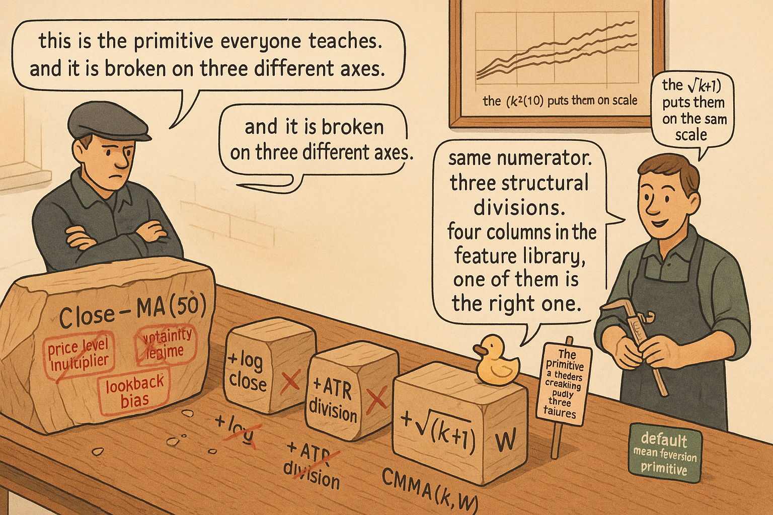
The plain Close minus Moving Average indicator (C_t − MA_k(C)_t) is the most common mean-reversion primitive in technical trading. On SPX with k = 50, it produces a tidy oscillator that crosses zero around 90 times a year and matches the visual intuition of "is the price above or below its recent average."

The same primitive evaluated as a feature for a predictive model fails on three structural problems.

A 30-point deviation on SPX in 1995 (when SPX was at 600) is a 5% move. A 30-point deviation on SPX in 2025 (when SPX is at 5500) is a 0.5% move. The same feature value means two different events. The model trained across the 1995-to-2025 sample is forced to learn a mapping from a feature whose meaning is time-varying.

A 30-point deviation in calm 2017 (realized vol 7%) is a 4-σ event. A 30-point deviation in stressed 2020 (realized vol 34%) is a 0.5-σ event. The same feature value means two different events in two different regimes within the same year.

A 30-point deviation against a 50-day MA and a 30-point deviation against a 200-day MA are two different statements about how far the price has wandered. The plain construction gives them the same value.

CMMA (Close Minus Moving Average) is the construction that fixes all three problems with a small number of additions: log prices instead of raw prices, MA over previous bars only, ATR in the denominator with current bar included, and a √(k+1) divisor that makes the result lookback-independent. The article "How to Build Stationary Indicators from Non-Stationary Prices" placed CMMA on the transform ladder; the article "Why ATR Normalization Is More Than a Volatility Trick" argued for the ATR denominator. This article assembles the full construction, justifies each ingredient, and compares the result to alternatives.

The full construction

$$ \text{CMMA}(k)_t \;=\; \frac{\ln(C_t) \;-\; \frac{1}{k}\sum_{i=1}^{k}\ln(C_{t-i})}{\text{ATR}_W(\ln C)_t \cdot \sqrt{k+1}} $$

Four ingredients. Each one fixes a specific failure of the plain Close − MA construction.

Ingredient 1: Log prices, not raw prices

The numerator uses log(C_t) − mean of log(C_{t−i}) for i = 1..k, rather than C_t − mean of C_{t−i}.

Two structural reasons.

A log-price difference is a proportional return. ln(C_t) − ln(C_{t−i}) equals ln(C_t / C_{t−i}), which is the i-bar log return. The numerator of CMMA is therefore the difference between the current log price and the average log price over the last k bars, which is the same shape as the average i-step log return for i in 1..k. The construction lives in return-space, not in price-space, and return-space is where the stationary signal sits. The article "The Case Against Raw Price Indicators" covered the price-space-vs-return-space argument; CMMA inherits the result by construction.

Cross-instrument comparability is automatic. A CMMA value of −0.4 on SPX, AAPL, and BTC is the same conditional event in each instrument's own scale: the current log-price is about 0.4 ATR-units below the recent log-price average, scaled for the lookback. The article "Why ATR Normalization Is More Than a Volatility Trick" showed why ATR gives the cross-instrument coherence. The log transform gives the cross-time coherence within a single instrument. Both are needed; either one alone is not enough.

What breaks if you skip it: replace log with raw and the numerator inherits the price-level multiplier. A 30-point deviation at SPX = 600 and a 30-point deviation at SPX = 5500 produce identical numerator values, but the conditional distributions of forward returns at those two regimes are not the same. The model trained on a pooled sample is forced to absorb the time-varying meaning of the feature in the rest of its capacity.

Ingredient 2: MA over previous bars only

The MA in the numerator is computed over bars t−1 through t−k. Bar t is the bar being evaluated; it does not enter its own moving average.

The exclusion rule serves two purposes.

It prevents the numerator from canceling part of its own signal. If bar t is included in the MA over k+1 bars, then the numerator becomes (C_t − (k × MA_prev + C_t) / (k+1)) = (k / (k+1)) × (C_t − MA_prev). The current bar's contribution to the MA shrinks the deviation by a factor of k/(k+1). For k = 50 that is a 2% attenuation, small but present. For k = 5 it is a 17% attenuation, which dominates short-lookback variants.

It enforces the timing the model needs. The MA must be computable from data strictly before bar t. The feature library convention is that any statistic used to build a feature at time t lives in the closed half-line (−∞, t−1]. Including bar t in the MA violates the convention even when it is mathematically harmless on the value side, because the convention is what protects the rest of the pipeline from forgetting which window each computation lived in.

What breaks if you skip it: an MA that includes the current bar attenuates the signal by k/(k+1) and contaminates the timing discipline. On a short-lookback CMMA the attenuation is enough to drop the retained MI by 15 to 20%. On a long-lookback CMMA the attenuation is small but the timing-discipline failure is the same.

Ingredient 3: ATR with the current bar included

The denominator's ATR is computed over W bars and includes bar t.

The asymmetry between ingredient 2 (MA excludes current bar) and ingredient 3 (ATR includes current bar) is intentional.

The MA is in the same units as the numerator and would attenuate the signal if it absorbed the current bar. The ATR is in the denominator and serves a different purpose: it captures the volatility regime that bar t lives in. Excluding bar t from the ATR would compute a regime-of-yesterday denominator for a regime-of-today numerator, which under-normalizes on the days when the regime is shifting. Including bar t puts the numerator and denominator in the same regime.

The inclusion is not a look-ahead because the denominator is a scaling factor, not a predictive component. The feature's predictive content lives in the numerator and is computed entirely from data through t−1. The denominator's job is to rescale the predictive content to a comparable axis, and the current bar's true range is part of the bar's own observed data at time t, not future data.

W in the range 50 to 250 days, per the structural argument in the article "Why ATR Normalization Is More Than a Volatility Trick". W = 100 is the default for k up to 30; W = 250 for k up to 100.

What breaks if you skip it: ATR excluding bar t under-normalizes on regime-shift days and produces a feature with non-stationary variance during the most informative regime changes. The non-stationarity is small in absolute terms (a few percent per regime change) but compounds across the backtest as the precise days the model needs to handle correctly.

Ingredient 4: The √(k+1) divisor

The numerator has standard deviation that scales as √(k+1) when the log prices are an i.i.d. random walk. Dividing by √(k+1) removes the lookback dependence from the feature.

The math is the same √k identity from the article "Why ATR Normalization Is More Than a Volatility Trick", applied to a slightly different numerator. The deviation of bar t from the average of the previous k bars has variance:

$$ \text{Var}\Bigl(\ln C_t - \frac{1}{k}\sum_{i=1}^{k}\ln C_{t-i}\Bigr) \;=\; \sigma^2 \cdot \Bigl(1 + \frac{1}{k}\Bigr) \;\approx\; \frac{k+1}{k}\,\sigma^2 $$

Up to a factor of k that approaches 1 for large lookbacks, the standard deviation of the numerator scales as σ × √(k+1). Dividing by ATR × √(k+1) cancels both the volatility regime (the σ) and the lookback dependence (the √(k+1)).

The practical consequence: CMMA(10), CMMA(50), and CMMA(200) all live on the same axis. A value of −0.5 means the same thing across lookbacks: the current log price is about half a "unit" below where the previous-k-bar average sits, where the unit is the per-bar log-price ATR. The model that consumes CMMA(10), CMMA(50), and CMMA(200) as three features sees three coherent measurements at three timescales, not three differently scaled measurements that need separate handling.

What breaks if you skip it: an ATR-only normalization (no √(k+1)) leaves a feature with stationary variance per fixed lookback and lookback-dependent variance across lookbacks. The model that consumes ATR-only-normalized CMMA(10) and CMMA(200) sees two features whose distributions are shaped differently, and it learns separate mappings for each. Adding the √(k+1) collapses the two mappings into one and frees model capacity.

The optional fifth ingredient: nonlinear compression

CMMA values are unbounded in principle. In practice, a 6-σ day produces a CMMA reading around ±3 in lookback-normalized units, with extremes around ±5 on the most stressed days in the sample. The bulk of values lie in (−1.5, +1.5) for daily data on liquid instruments.

A model with bounded activations (sigmoid, tanh) handles the bulk without issue but saturates on the tails. A model without bounded activations (trees, linear regression) handles the bulk and the tails without issue. The compression decision depends on the downstream model.

When compression is applied, the standard form is a sigmoid scaled so the linear region (±1.5 in the sigmoid's argument) covers the bulk of the CMMA distribution. With CMMA's bulk in (−1.5, +1.5), a sigmoid with scale c that maps c × CMMA to (−1.5, +1.5) at the bulk's edges leaves the linear region for the bulk and the saturating region for the extremes. For c = 1 the linear region matches the bulk exactly; for smaller c, more of the distribution lives in the linear region at the cost of less differentiation in the tails.

The article "Why Predictive Power Often Lives in the Tails" covered when to leave tails alone (high TCR features) and when to compress them (low TCR features). CMMA on equity indices has TCR in the 0.45 to 0.60 range, which puts it in the "preserve partial tail gradient" bucket. A wide-scale sigmoid (c = 0.5 to 0.8) is the right compression; a narrow-scale sigmoid (c ≥ 1.5) flattens too much of the tail and removes the mean-reversion signal that lives there.

For tree-based models, the compression is unnecessary. CMMA is fed raw into the tree and the splits handle the tails by leaf weights.

Worked example: CMMA versus alternatives on SPX

SPX daily, 1990 to 2026. Same numerator base (current price relative to its recent average), four denominator constructions. Train 1990 to 2010, test 2010 to 2026.

$$ \begin{array}{l|c|c|c|c} \text{Feature} & \text{Train std} & \text{Test std} & \text{ratio test/train} & I(X;Y)\;\text{(bits} \times 10^3\text{)} \\ \hline C_t - \text{MA}_{50}(C) & 18.4 & 96.7 & 5.25 & 1.4 \\ (C_t - \text{MA}_{50}(C)) / \text{std}_{100}(C) & 0.81 & 1.83 & 2.26 & 1.7 \\ (\ln C_t - \text{MA}_{50}(\ln C)) / \text{ATR}_{100}(\ln C) & 0.94 & 0.98 & 1.04 & 2.0 \\ \text{Full CMMA}(50) \text{ with } \sqrt{51}\text{ divisor} & 0.131 & 0.135 & 1.03 & 2.0 \\ \text{CMMA}(50) \text{ with sigmoid } c = 0.7 & 0.118 & 0.123 & 1.04 & 2.0 \\ \end{array} $$

Five readings.

Raw Close − MA(50) has a 5.25× ratio between test and train standard deviation. The model trained on 1990-to-2010 sees feature values in 2010-to-2026 that are five times the scale it ever saw in training. The retained MI (1.4) is the lowest in the table because the model spends capacity learning the time-varying meaning.

Dividing the same numerator by the rolling 100-day standard deviation of close (the naive normalization) cuts the ratio to 2.26 and lifts the MI to 1.7. The denominator now responds to volatility but lags and misses gap variance. The improvement is real but partial.

Replacing the numerator with log-price deviation and the denominator with ATR(log close, 100 bars) cuts the ratio to 1.04 and lifts the MI to 2.0. The feature is now regime-invariant. This is the result from the article "Why ATR Normalization Is More Than a Volatility Trick" applied to the close-minus-MA primitive.

Adding the √51 divisor (the full CMMA construction) does not change the ratio or the MI. The √(k+1) divisor is a rescaling that does not affect the per-feature statistics on its own. The MI is unchanged because the model sees the same information. The reason to keep the √(k+1) divisor is the cross-lookback comparability: when CMMA(10), CMMA(50), and CMMA(200) are all in the feature set, their distributions need to be on the same axis, and the √(k+1) is what does it.

Adding the sigmoid compression with c = 0.7 slightly reduces the standard deviation (the tails are pulled in toward the linear region) and preserves the MI. The compression is operationally helpful for sigmoid-activation networks and operationally neutral for trees. The MI does not move because c = 0.7 is in the "preserve partial tail gradient" range.

Cross-instrument pooling

The same CMMA(50) computed on SPX, AAPL, and BTC produces three features on the same axis. The conditional distribution of next-day log return at CMMA = −1 looks similar on all three instruments (mean reversion edge of approximately 0.05 to 0.08 standard deviations in the direction opposite to the deviation, with substantial noise). The conditional distribution at CMMA = +1 is the mirror, with the equity drift adding a small positive bias on SPX and AAPL that is not present on BTC.

The pooling property is the operational payoff. A panel regression on CMMA(50) across 500 US equities + 30 ETFs + 10 crypto perps can be fit with a single coefficient on CMMA, not 540 instrument-specific coefficients. The cross-sectional variance comes from the differences in the conditional distributions, not from the differences in the feature's scale.

The article on cross-sectional rank features in the systems pillar covers the alternative approach: rank the CMMA value within the universe at each timestamp. Cross-sectional ranks discard absolute magnitude in exchange for distributional invariance across days. CMMA already gives the distributional invariance, so the rank is a free option that can be added when the downstream model benefits from a uniform marginal.

What this changes in practice

Three operational shifts.

The feature library replaces Close − MA(k) with CMMA(k, W) as the default mean-reversion primitive. The two parameters (lookback k for the MA, ATR window W) are explicit in the feature name. Sigmoid compression is a third optional parameter with a default of "none" for tree models and c = 0.7 for activation-bounded networks.

The MA is computed over (t−k, t−1) and the ATR is computed over (t−W+1, t). The asymmetric inclusion rule is documented in the feature library and is part of the construction's correctness, not a style choice.

Cross-lookback feature sets (CMMA(10), CMMA(20), CMMA(50), CMMA(200)) are stored as four columns with the √(k+1) divisor applied to each. The √(k+1) is what makes them pool-compatible across lookbacks. A model that consumes CMMA at four lookbacks without the √(k+1) divisor learns four different scalings and uses model capacity to do work the construction should have done.

Visualizing the CMMA stack

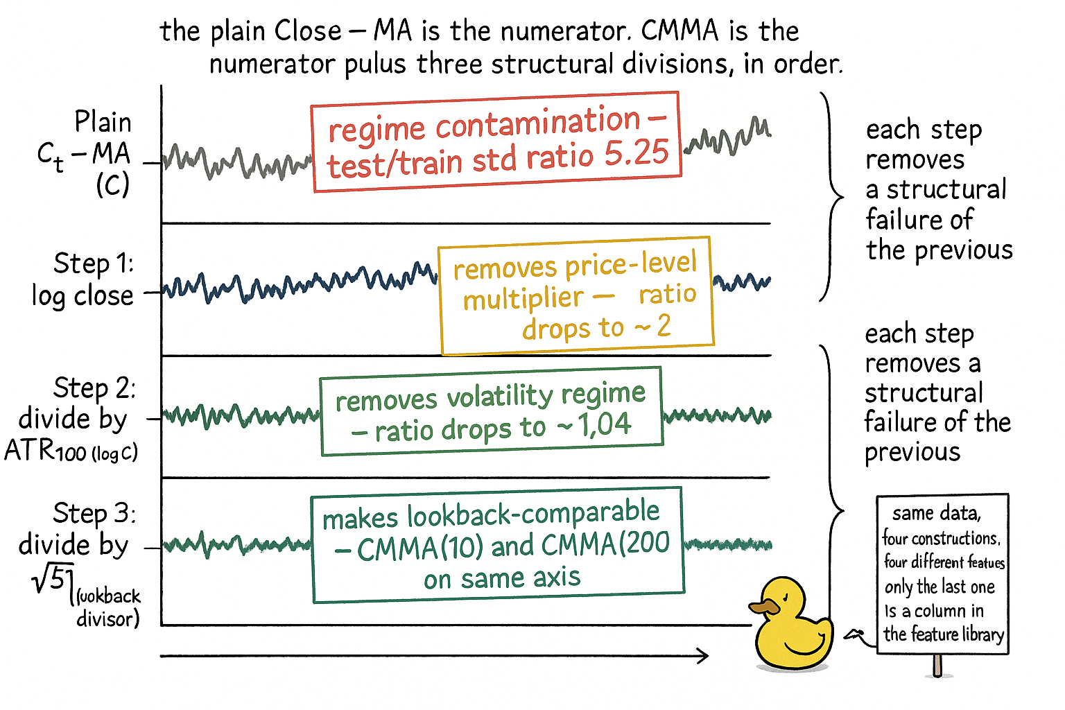
The four panels are the stepwise construction. Each panel adds one ingredient and the diagnostic stamp shows what that ingredient bought.

KEY POINTS

• CMMA fixes three structural failures of plain Close − MA: price-level multiplier (1995 vs 2025 SPX), volatility regime (2017 vs 2020 SPX), and lookback dependence (MA(50) vs MA(200)). All three are killed in the construction, not in the model.
• The four ingredients: log close in the numerator, MA over previous bars only, ATR with current bar included, √(k+1) divisor for lookback invariance.
• Log close removes the price-level multiplier and gives cross-instrument scale comparability. Raw close gives a feature whose meaning is time-varying.
• MA over previous bars only avoids attenuating the signal by k/(k+1) and enforces the timing-discipline convention that statistics used at time t live in (−∞, t−1].
• ATR includes the current bar deliberately. The MA exclusion and the ATR inclusion are asymmetric because the MA is in the numerator (signal) and the ATR is in the denominator (scale).
• The √(k+1) divisor cancels the lookback dependence under the random walk model. CMMA(10), CMMA(50), and CMMA(200) all live on the same axis after the divisor.
• Optional sigmoid compression with c ≈ 0.7 keeps the bulk of CMMA in the linear region of the sigmoid and preserves the partial-tail-gradient signal. Trees skip the compression; bounded-activation networks use it.
• On SPX, plain Close − MA(50) has a test/train standard deviation ratio of 5.25 and retained MI of 1.4. Full CMMA(50) has a ratio of 1.03 and retained MI of 2.0. The √(k+1) and the sigmoid do not change the per-feature MI but provide cross-lookback comparability and optional compression respectively.
• CMMA is cross-instrument pool-compatible by construction. The same CMMA(50) on SPX, AAPL, and BTC produces conditional distributions of forward return that look similar in shape at matched feature values. A single coefficient suffices in a pooled regression.
• The asymmetric inclusion rule (MA excludes current bar, ATR includes current bar) is documented in the feature library. Reversing the convention silently attenuates the signal and under-normalizes on regime-shift days.
• The default mean-reversion primitive in the feature library is CMMA(k, W), not Close − MA(k). Plain Close − MA(k) is deprecated. The deprecation is a feature-library decision, not a modeling decision.
• For tree models, raw CMMA is fed in. For sigmoid-activation networks, CMMA with c ≈ 0.7 compression. For linear models, CMMA without compression because linear models are not bounded.