2.14 Taming Indicator Tails with Sigmoid Transforms
A wrong-scale sigmoid destroys the signal. Center on training median; scale α so IQR lands in the linear region (α≈1.2 for tanh). On SPX Range/Close, α=1.2 lifts AUC 0.503 → 0.519.
A common reflex: indicator has a heavy-tailed bell shape (Shape 2 from the article "Why Indicator Histograms Matter"), so apply tanh to the raw values. The histogram comes back tight and bounded in (−1, +1). R/IQR drops from 12 to 1.4. The diagnostic says clean.
Refit the model. AUC drops from 0.516 to 0.504. The naive tanh did not just compress the tails. It also collapsed the central body of the distribution into the steep part of the sigmoid, where small differences in the raw indicator produce small differences in the transformed value. The signal in the body was lost to the sigmoid's slope, and the signal in the tails was lost to its saturation. The transform took the whole feature with it.
The cure is not a different sigmoid. The cure is the same sigmoid, applied correctly. The rule: scale the raw values so the bulk of the distribution lives in the linear region of the sigmoid (the region where the sigmoid behaves like a straight line) and only the genuine tail outliers reach the saturating knees. A correctly scaled sigmoid preserves the body's signal at near-linear resolution and clips the tails. An incorrectly scaled sigmoid does both jobs wrong.
This article is the recipe. Four construction steps, three family choices (tanh, normal CDF, logistic), one tuning parameter (the linear-region scale), and a worked example on a heavy-tailed feature where the correct scale recovers the AUC the naive scale destroyed.
The decision of when to use a sigmoid (low-TCR features with heavy tails) versus when to skip it (high-TCR features where the tails carry signal) is the subject of the article "Why Predictive Power Often Lives in the Tails". This article assumes you already know the feature is low-TCR and the sigmoid is the right transform. The question is how to scale it.
The four-step construction
Step 1: Center the distribution. The sigmoid family operates around zero. A feature with a non-zero center pushes its bulk off-center in the sigmoid's argument and the linear region no longer covers the bulk. Subtract the in-sample median:
$$ X^c_t \;=\; X_t \;-\; \text{median}_{\text{train}}(X) $$
The median is preferred over the mean because the in-sample mean is contaminated by the same tails the sigmoid is meant to tame. Use the training-sample median, not the rolling median, because the rolling median changes the centering as a function of t and breaks the sigmoid's interpretation.
Step 2: Measure the bulk's spread. The bulk is the central 50% to 80% of the distribution. The IQR is the standard measurement and is robust to the tails:
$$ s \;=\; \text{IQR}_{\text{train}}(X^c) \;=\; X^c_{[0.75]} - X^c_{[0.25]} $$
The standard deviation can be used instead of IQR when the indicator has light tails. For heavy-tailed indicators (the case this article addresses), IQR is the correct choice because a single outlier inflates std and silently rescales every observation by the wrong factor. The article "Range/IQR: A Simple Test for Indicator Tail Problems" covered the IQR's robustness rationale.
Step 3: Scale the centered values so the bulk lands in the linear region. The HTAN function (hyperbolic tangent) is linear within roughly ±1.5 in its argument. The normal CDF is linear within roughly ±1.0. The logistic function is linear within roughly ±1.0. To map the central 80% of the distribution into the linear region, multiply the centered values by a scale factor:
$$ Y_t \;=\; \tanh\!\Bigl(\,\alpha \cdot \frac{X^c_t}{s}\,\Bigr), \qquad \alpha \approx 1.0 \text{ to } 1.5 $$
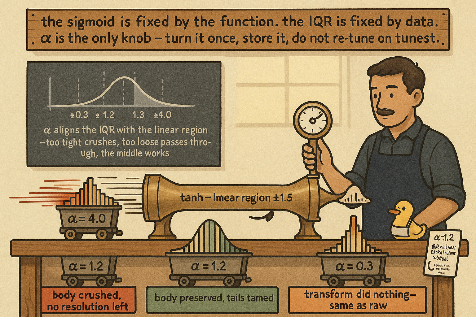
For tanh, α = 1.2 puts the IQR boundaries at ±1.2 in the sigmoid's argument, which sits inside the linear region (±1.5). For the normal CDF, α = 0.8 puts the IQR boundaries at ±0.8, which sits inside its linear region (±1.0). The α parameter is the single tuning knob that controls how aggressively the sigmoid compresses the tails.
Step 4: Optionally rescale the output. Tanh outputs to (−1, +1). Normal CDF outputs to (0, 1). Logistic outputs to (0, 1). For downstream consumers that want a (−1, +1) output, the normal CDF and logistic need a shift and rescale (output × 2 − 1). For consumers that want a (0, 1) output, tanh needs (output + 1) / 2. The output rescaling does not change the feature's information content; it only changes the axis label.
The full construction in one line:
$$ \tilde{X}_t \;=\; \tanh\!\Bigl(\,\alpha \cdot \frac{X_t - m}{s}\,\Bigr), \quad m = \text{median}_{\text{train}}(X), \quad s = \text{IQR}_{\text{train}}(X) $$
The training-sample statistics m and s are stored with the feature and held fixed in production. Re-computing them on test data is the look-ahead anti-pattern the article "How to Build Stationary Indicators from Non-Stationary Prices" catalogged.
The linear region rule
The sigmoid is approximately linear in a window around zero and saturating outside that window. The scaling rule operationalizes the "stay in the linear region" guidance with a specific quantile target.
Three operational targets, in order of aggressiveness:
Aggressive compression: α scaled so the in-sample 95th percentile of |X^c / s| lands at the edge of the linear region (±1.5 for tanh). The central 90% of the distribution is in the linear region and the top/bottom 5% are pulled toward the saturating knees. Equivalent to α ≈ 0.6 to 0.8.
Moderate compression (default): α scaled so the in-sample 90th percentile lands at the edge of the linear region. The central 80% is linear; the top/bottom 10% are in the knees. Equivalent to α ≈ 1.0 to 1.2.
Mild compression: α scaled so the in-sample 75th percentile (the IQR boundary) lands at the edge of the linear region. The central 50% is linear; the rest is in the knees. Equivalent to α ≈ 1.5 to 2.0. Useful when the TCR is borderline and partial tail preservation matters.
For a typical low-TCR heavy-tailed-bell indicator on equity indices, moderate compression (α ≈ 1.0 to 1.2) is the default. The aggressive variant is reserved for indicators known to have a few data errors mixed into the tail. The mild variant is for indicators that almost qualified as high-TCR but still need some tail protection.
The choice of α is a structural parameter of the feature, not a hyperparameter of the model. It is set once at the feature design stage, stored with the feature definition, and not re-optimized on the backtest.
Sigmoid family options
Three sigmoid functions appear in the indicator-design literature. They differ in details that matter for specific downstream consumers.
Hyperbolic tangent (tanh). Output range (−1, +1). Linear region ±1.5 in argument. Symmetric around zero. Derivative at zero is 1 (so the linear region has slope 1). The default for indicators that already live on a signed axis (oscillators, mean-reversion features, normalized differences).
$$ \tanh(x) \;=\; \frac{e^x - e^{-x}}{e^x + e^{-x}} $$
Normal CDF (Φ). Output range (0, 1). Linear region ±1.0 in argument. Symmetric around the midpoint (Φ(0) = 0.5). Derivative at zero is 1/√(2π) ≈ 0.4 (linear region has slope ≈ 0.4). Often preferred when the downstream model is a logistic regression or a probability-output model, because the CDF interpretation aligns with probability outputs.
Logistic. Output range (0, 1). Linear region ±1.0 in argument. Symmetric around the midpoint. Derivative at zero is 0.25. Computationally cheaper than the normal CDF (no error function required). Behaves almost identically to tanh after the linear shift Y = 2 × logistic − 1.
For practical purposes, tanh and the rescaled logistic are interchangeable. The normal CDF is the right choice only when there is a structural reason to want a CDF interpretation (Bayesian models, probabilistic ensembles). Pick tanh by default; pick the normal CDF when the downstream model is built around probabilities.
Worked example: SPX Range/Close, three sigmoid scalings
SPX daily, 1990 to 2026. Feature: same-bar Range divided by Close (a Shape 2 heavy-tailed bell, low TCR ≈ 0.30 because the signal lives in the body, not the extreme range days). Train 1990 to 2010, test 2010 to 2026.
Four candidate features. The raw feature, then three tanh variants with different α scaling.
$$ \begin{array}{l|c|c|c|c} \text{Feature} & \text{R/IQR} & \alpha & \text{Test AUC} & I(X;Y) \times 10^3 \\ \hline \text{Raw Range/Close} & 12.4 & - & 0.503 & 1.1 \\ \tanh(\alpha \cdot (X-m)/s),\; \alpha = 4.0 \text{ (over-tight)} & 1.05 & 4.0 & 0.504 & 1.0 \\ \tanh(\alpha \cdot (X-m)/s),\; \alpha = 1.2 \text{ (moderate)} & 1.42 & 1.2 & 0.519 & 2.0 \\ \tanh(\alpha \cdot (X-m)/s),\; \alpha = 0.3 \text{ (over-loose)} & 8.9 & 0.3 & 0.508 & 1.4 \\ \end{array} $$
Four readings.
The raw feature has R/IQR = 12.4 and test AUC barely above the coin flip. The model trained on the 1990-to-2010 distribution sees test-period tail values the training set did not contain, and the loss function gets dominated by a few large observations. The MI is real (1.1) but the model cannot consume it.
The over-tight sigmoid (α = 4.0) puts the IQR boundary at ±4.0 in the tanh argument, where tanh has already saturated. The bulk of the distribution is mapped into the saturating region. Differences in the raw feature in the body produce almost no difference in the transformed feature. The histogram looks clean (R/IQR = 1.05, the tightest bound the diagnostic recognizes), but the AUC and MI confirm the transform destroyed the signal it was meant to preserve.
The moderate sigmoid (α = 1.2) puts the IQR boundary at ±1.2 in the tanh argument, which is inside tanh's linear region (±1.5). The body of the distribution is approximately linear after the transform; the tails are pulled into the knees. The R/IQR comes back at 1.42, the AUC lifts to 0.519, and the MI lifts to 2.0 (higher than the raw because the model can now consume what the transform exposes). This is the correct scale.
The over-loose sigmoid (α = 0.3) puts the IQR boundary at ±0.3 in the tanh argument, which is so close to zero that the whole sigmoid behaves like a linear function on this data. The R/IQR drops only to 8.9; the tails are barely touched. The AUC and MI improve over raw but not enough to justify the transform. The over-loose variant is the same as not transforming.
The middle option is the only one that produces a useful feature. The two failure modes (over-tight and over-loose) bracket it on both sides.
When not to sigmoid
The article "Why Predictive Power Often Lives in the Tails" covered the case structurally. The decision rule, restated for the sigmoid construction:
| TCR | R/IQR | Action |
|---|---|---|
| Below 0.3 | Above 5 | Sigmoid with moderate α — body holds signal, tails are noise |
| 0.3 to 0.5 | Above 5 | Sigmoid with mild α (≥ 1.5) — preserve partial tail gradient |
| 0.5 to 0.6 | Above 5 | Wide-scale sigmoid or fourth-root — tails carry partial signal |
| Above 0.6 | Above 5 | Winsorize at 99.5%, do not sigmoid — tails carry primary signal |
| any | Below 3 | No transform — feature is already in shape |
A sigmoid applied to a high-TCR feature is the worst case. It removes the tail differentiation that carried the signal and leaves the body that was carrying noise. The article's opening example (sigmoid on TCR = 0.78 realized vol, AUC drops from 0.518 to 0.506) shows the magnitude.
Anti-patterns
Four patterns that produce a feature that looks sigmoid-compressed but is functionally broken.
Sigmoid on an uncentered distribution. A one-sided exponential (Shape 3 from the article "Why Indicator Histograms Matter") has its mode at zero and no mass on the negative side. Subtracting the median moves the mode to the negative side but the distribution is still asymmetric. The sigmoid applied to such a feature compresses the upper tail and leaves the lower side functionally untouched. The right transform for one-sided distributions is a root or a log, not a sigmoid.
Sigmoid on a bimodal distribution. Bimodal (Shape 5) features have two modes with a valley between them. The sigmoid maps the valley to the linear region and the two modes to opposite knees. The output looks unimodal at the histogram level but the conditional structure (the two regimes that produced the bimodality) is now hidden. The article "Why Indicator Histograms Matter" covered the regime-split fix; the sigmoid is not it.
Sigmoid stacked on a log transform. The log is a transform from the root/log family that already compresses the tail. Applying tanh on top of log values produces double compression: the log handles the multiplicative tail and the sigmoid handles the residual additive tail. The combined transform's behavior is almost always over-tight on the body and adds no benefit over either transform alone. Pick one family, not both.
Sigmoid with full-sample statistics. Computing m and s using the full training+test sample is the look-ahead anti-pattern the article "How to Build Stationary Indicators from Non-Stationary Prices" catalogged. The bound that the sigmoid imposes is a function of m and s, and m and s computed on the test set are not available in production. Use training-sample-only statistics, and update them forward in the walk-forward.
Visualizing the scale parameter
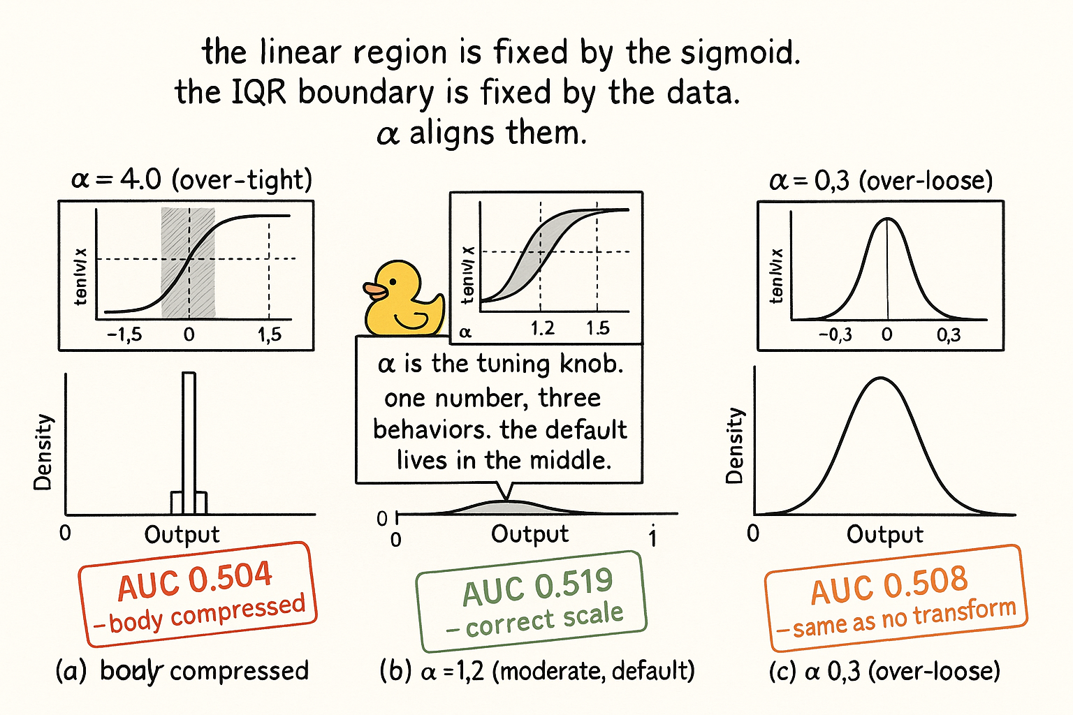
The three panels are the scale-parameter diagnostic. Same data, same sigmoid family, three α values, three feature qualities. Only the middle one survives.
What this changes in practice
Three operational shifts.
Sigmoid transforms in the feature library carry α as part of the feature identifier. "Range_over_close_tanh_alpha_1.2" and "Range_over_close_tanh_alpha_0.8" are different features. The α is stored as metadata, not as a model hyperparameter.
The α default for moderate compression is set to 1.2 for tanh, 0.8 for normal CDF, and 1.0 for logistic. These defaults map the in-sample IQR boundary to the edge of each sigmoid's linear region. Departures from the default require justification (recorded in the feature audit) tied to the TCR of the feature.
The sigmoid m and s are stored with the feature definition, computed from training-window data only, and updated forward in walk-forward without re-fitting on the held-out window. The audit checks that the test-period feature distribution lies within the training-period support after the transform; a > 5% test-period saturation rate on the bounded output triggers a feature-drift review.
KEY POINTS
- The naive sigmoid (tanh applied to raw values, no scaling) compresses the body of the distribution into the saturating knees and destroys the signal that the body carried. The AUC penalty is typically 0.005 to 0.015 per feature.
- The four-step construction: subtract the training-sample median (center), measure the IQR (spread), scale by α so the IQR boundary lands inside the sigmoid's linear region, apply the sigmoid.
- The linear region of tanh is ±1.5 in argument. The linear region of the normal CDF is ±1.0. The linear region of the logistic is ±1.0. Scale the input so the bulk of the distribution lives inside that region.
- α = 1.2 is the moderate-compression default for tanh. It maps the in-sample IQR boundary to ±1.2 in the tanh argument, leaving 80% of the distribution in the linear region and the top/bottom 10% in the knees.
- α below 0.5 leaves the tails untouched (over-loose). α above 2.5 collapses the body into the knees (over-tight). Both failure modes are diagnosable from the histogram of the transformed feature.
- tanh, the normal CDF, and the logistic are interchangeable for most purposes. The normal CDF is preferred when the downstream model is probabilistic. tanh is the default everywhere else.
- The IQR is preferred to the standard deviation as the spread measure because a single tail outlier inflates the std and silently rescales the entire feature by the wrong factor.
- The median is preferred to the mean as the center because the in-sample mean is contaminated by the same tails the sigmoid is being applied to remove.
- The m and s used in the transform are computed from training-window data only. Full-sample statistics leak the test distribution into the feature definition.
- A sigmoid on a high-TCR feature (TCR above 0.6) destroys the tail differentiation that carried the signal. Use winsorization instead. The decision matrix maps TCR and R/IQR to the correct transform.
- A sigmoid on a one-sided exponential (Shape 3) is the wrong family entirely. Use a root or a log. A sigmoid on a bimodal feature (Shape 5) hides the regime structure. Split into regime-conditional features instead.
- Stacking a sigmoid on top of a log is double compression with no benefit. Pick one family per feature, not both.
- On SPX Range/Close (low TCR), the raw feature has test AUC 0.503 and the over-tight α = 4.0 sigmoid has test AUC 0.504. The correctly scaled α = 1.2 sigmoid has test AUC 0.519 and MI 2.0, both higher than the raw because the model can now consume the body without the tail-leverage problem.
References
- Statistically Sound Indicators for Financial Market Prediction - Timothy Masters (Amazon)
- Cycle Analytics for Traders - John Ehlers (Amazon)
- Forecasting Financial Time Series Using Hybrid ARIMA-ANN Models
- Hierarchical Endogenous Market-State Representation for Financial Time Series
- Digital Signal Processing, System Analysis and Design, 2nd Edition
- Automatic Outlier Rectification via Optimal Transport - arXiv
- Rocket Science for Traders: Digital Signal Processing Applications
- Financial Time-Series Forecasting: Towards Synergizing ... - arXiv
- Taming Vision Priors for Data Efficient mmWave Channel Modeling
- Introduction to Real-Time Digital Signal Processing