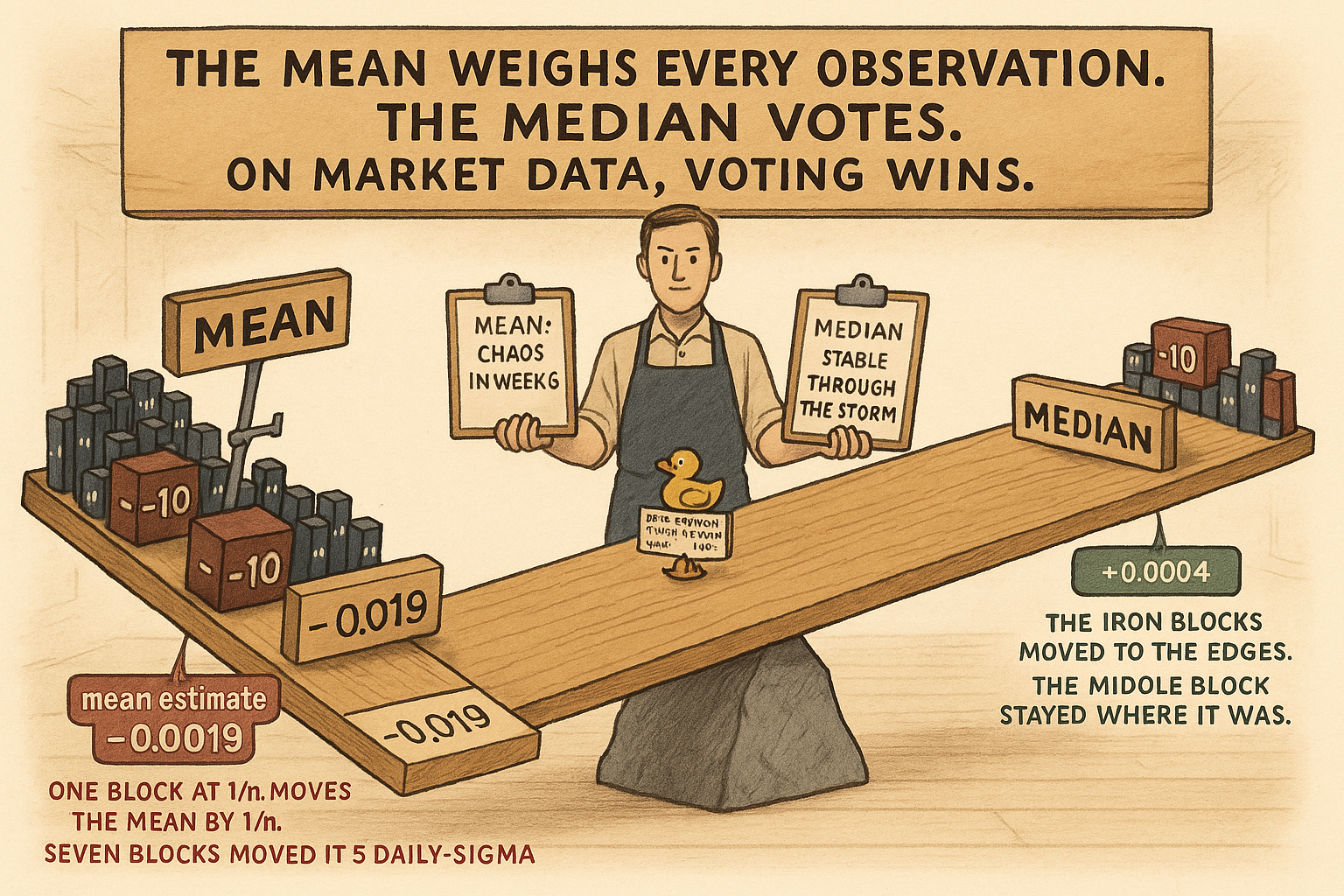
Compute the rolling 100-day mean of SPX daily log return on February 28, 2020. The value is +0.0004 (roughly 10% annualized). Compute the same statistic on March 20, 2020, three weeks later. The value is −0.0019 (roughly −48% annualized). The estimator dropped by 5 standard deviations in 14 trading days. The "estimate of the central tendency" of SPX daily returns moved by half a year's worth of nominal return because seven days in March produced double-digit moves and each one entered the average at weight 1/100.

Compute the rolling 100-day median of the same series. On February 28: +0.0006. On March 20: +0.0004. The median moved by 0.0002, or roughly 0.4 of a daily standard deviation. The crash days entered the sorted list but did not change which day sat at the 50th percentile of the window.

The mean is the wrong estimator of the center for any trading feature whose distribution has tails. The median is the right estimator. The same logic applies up the L1 / L2 ladder: MAD and IQR beat standard deviation for spread measurement, Spearman beats Pearson for correlation on heavy-tailed pairs, LAD beats OLS for rolling regression on noisy market series, and rolling median filters beat moving averages for smoothing volume, range, and other outlier-prone primitives.

This article catalogs the five places L1 statistics beat L2 statistics in trading feature design, gives the structural reason (breakdown point and heavy-tail efficiency), and names the counter-cases where the mean is still correct. The operational rule: if the indicator does not have outliers use mean; if it has outliers use median. Most trading features have outliers. The mean is the default that should have been the median.

The breakdown point

The breakdown point of an estimator is the smallest fraction of observations that, when corrupted arbitrarily, can drive the estimator to an arbitrary value.

$$ \text{breakdown}(\text{mean}) \;=\; \frac{1}{n}, \qquad \text{breakdown}(\text{median}) \;=\; 0.5 $$

A single observation can push the mean to any value. Half the observations must be corrupted to push the median by more than a fixed amount. On a 100-bar rolling window, one large outlier shifts the mean by 1% of its full value, the same outlier shifts the median by 0 (it does not change which observation sits at the sorted middle).

Three related estimators share the median's breakdown property:

The median absolute deviation (MAD = median of |x_i − median(x)|) has breakdown 0.5. The standard deviation has breakdown 0 (a single observation squared dominates the sum).

The IQR (75th percentile minus 25th percentile) has breakdown 0.25. The range has breakdown 1/n.

Spearman's rank correlation has breakdown 0.5 for the rank computation (a single pair-swap moves the rank correlation by at most 2/n). Pearson's product-moment correlation has breakdown 0 because the products in the numerator are unbounded in the raw observations.

Breakdown is not a niche concern on trading data. SPX daily returns have a kurtosis around 25. A 5-sigma daily move appears 5 to 10 times per decade. On any 100-bar window that contains one such day, the mean and the std are 5 to 30% off their "no-outlier" values; the median and MAD are within 1 to 2% of theirs.

Five places L1 beats L2

Application 1: centering a feature for downstream transformation. The article "Taming Indicator Tails with Sigmoid Transforms" used the training-sample median as the centering statistic. The reason is exactly the breakdown argument: the in-sample mean is contaminated by the same tails the sigmoid is meant to tame. Centering by the mean shifts the bulk of the distribution by an amount proportional to the contamination, which the sigmoid then maps off-center. Centering by the median places the bulk's symmetric center at zero regardless of the tails.

Application 2: spread measurement for normalization. The article "Range/IQR: A Simple Test for Indicator Tail Problems" and the article "How to Build Stationary Indicators from Non-Stationary Prices" both used IQR over standard deviation for variance-scaling normalizations. The MAD is the closer L1 analogue of the standard deviation:

$$ \text{MAD}(X) \;=\; \text{median}\bigl(|X_i - \text{median}(X)|\bigr) $$

For Gaussian data, the standard deviation equals 1.4826 × MAD. For heavy-tailed data, the standard deviation is dragged up by the tails and overestimates the bulk's spread; the MAD measures the bulk's spread directly. A spread-normalization divides by MAD (or by IQR, which is 1.35 × MAD for Gaussian data and a similar-magnitude robust statistic in general). Dividing by std on a heavy-tailed feature under-normalizes the body and over-normalizes the tails.

Application 3: smoothing outlier-prone primitives. Volume, true range, absolute return, and intraday range are heavy-tailed by construction. A moving average of these primitives carries the outlier days at weight 1/W for W bars after the day, dragging the smoothed value upward for a 1/W-decaying duration. A rolling median of the same primitives kills the spike immediately: as soon as the outlier exits the sorted middle of the window, the median returns to baseline.

$$ \text{rolling\_median}(X, W)_t \;=\; \text{median}\bigl(X_{t-W+1},\,\ldots,\,X_t\bigr) $$

Rolling median filters have a second property worth naming: they preserve edges. A step change in the underlying signal (say, a regime shift in volume after an index inclusion) appears as a step in the rolling median. A moving average of the same step rounds the corners over W bars. For smoothing primitives that can have genuine step changes mixed with spikes, the median is structurally the right filter.

Application 4: correlation on heavy-tailed pairs. Pearson correlation between two return series, two volume series, or any pair where both legs are heavy-tailed is dominated by a small number of joint-tail observations. One co-movement on a crash day can push Pearson correlation from 0.3 to 0.7 and back again over a 100-bar window.

Spearman rank correlation operates on the ranks of the observations, not the values. The crash-day pair becomes "rank 100 paired with rank 100" instead of "−10% paired with −8%". The contribution of the joint-tail observation is bounded above by the largest possible rank-product. Spearman's correlation moves slowly and stably, which is what is wanted for any feature built on rolling correlation. Kendall's τ has the same property and is preferred for very small samples.

Application 5: rolling regression for prediction-deviation features. Indicators of the form "predicted − actual" built from rolling regressions (Detrended RSI, cross-market deviation indicators) suffer when the regression is fit with OLS on heavy-tailed data. One outlier pair pushes the OLS slope by a multiple of the noise scale, and the resulting "deviation" is dominated by the regression's own fitting error rather than the structural deviation it was meant to detect.

LAD (least absolute deviations) regression and Huber regression replace the squared-error loss with an L1 or robust loss. The fitted slope is no longer dominated by single-pair outliers; the deviation indicator measures the structural mispricing it was designed for. The cost is computational (LAD has no closed form and Huber needs iterative reweighting), and on modern hardware the cost is negligible for the rolling-window sizes used in feature engineering.

When the mean is correct

Three counter-cases where the mean is the right choice and the median is wasted robustness.

Light-tailed bell features. RSI(14) on SPX, Stochastic K(14), and other bounded-by-construction oscillators have R/IQR around 2 to 4 (per the article "Range/IQR: A Simple Test for Indicator Tail Problems"). The tails are not contaminated, the breakdown concern does not bite, and the mean is more efficient than the median on near-Gaussian data. Use the mean.

Additive aggregations. Computing the total realized variance over a window is a sum, and the sum's expected value is N × E[X²]. Replacing the sum with the median × N would be mathematically wrong. When the downstream computation requires the additive interpretation (portfolio P&L, total volume, integrated variance), the mean is the correct estimator regardless of tail behavior.

MSE-target downstream models. A model whose loss function is mean squared error implicitly treats the mean as the correct point estimate of the target. Using the median to center a feature consumed by an MSE-loss model creates a mild inconsistency between the feature's center and the model's loss-minimizing prediction. For most practical purposes the inconsistency is irrelevant (the model adjusts in the bias term), but for some loss-function variants (quantile regression, asymmetric losses) the centering should match the loss.

The decision rule: use the median when the distribution has tails and the downstream usage does not require the additive or MSE-aligned interpretation. Use the mean when the distribution is light-tailed or the additive interpretation is structurally required.

The efficiency cost is not what you think

A common objection: the median has only 64% efficiency of the mean on Gaussian data, so the median is a worse estimator. The objection is correct on Gaussian data. The objection misses the point on market data.

Statistical efficiency is measured relative to the variance of the estimator. For Gaussian data, the median's variance is (π / 2) × σ² / n ≈ 1.57 σ² / n, while the mean's variance is σ² / n. The median needs more observations to achieve the same precision.

For heavy-tailed data, the calculation reverses. The variance of the sample mean depends on the underlying variance, which is large on heavy-tailed distributions. The variance of the sample median depends on the local density at the median, which is the same for Gaussian and heavy-tailed bells (both have a smooth bulk around the center). On a Student's t-distribution with 3 degrees of freedom (kurtosis around 9, similar to many market features), the median's efficiency is roughly 1.5× the mean's. On a distribution with kurtosis 25 (SPX daily returns), the median's efficiency is 3× to 5× the mean's.

The relevant efficiency comparison for market features is on the actual distribution, not on a hypothetical Gaussian. On real distributions, the median is more efficient than the mean for most trading features whose downstream use only needs a center estimate. The Gaussian-efficiency penalty is a textbook artifact, not a real cost.

Worked example: SPX rolling center estimate through March 2020

SPX daily log returns, 100-bar rolling window. Three center estimators: mean, median, and 20% trimmed mean (a hybrid that drops the top and bottom 10% before averaging).

$$ \begin{array}{l|c|c|c|c} \text{Date} & \text{rolling mean} & \text{rolling median} & \text{20\% trimmed mean} & \text{notes} \\ \hline \text{2020-02-28 (pre-crash)} & +0.0004 & +0.0006 & +0.0005 & \text{light tails in window} \\ \text{2020-03-13 (mid-crash)} & -0.0011 & +0.0005 & -0.0001 & \text{6 large negative days in window} \\ \text{2020-03-20 (peak stress)} & -0.0019 & +0.0004 & -0.0003 & \text{worst readings} \\ \text{2020-04-30 (recovery)} & -0.0008 & +0.0007 & +0.0001 & \text{positive days re-entering} \\ \text{2020-06-30 (post-crisis)} & +0.0006 & +0.0008 & +0.0007 & \text{crash days still in window} \\ \end{array} $$

Three readings.

The rolling mean spikes downward by 5 daily-σ from February 28 to March 20, even though the underlying "central tendency" of SPX daily returns (whatever the true value is) did not change by anything close to that. The estimator absorbed seven extreme days at weight 1/100 each and reported a "center" that lived nowhere in the data's bulk.

The rolling median moved by 0.0002 over the same period. The seven extreme days entered the sorted window but did not change which day sat at the 50th percentile. The median's estimate of the center is robust to the crash and is the operationally useful number.

The 20% trimmed mean is the intermediate option. It throws away the top and bottom 10% of the window before averaging the rest. The trimmed mean is more efficient than the median on heavy-tailed but not pathological distributions and moves slightly with the crash (the bulk shifts down by a fraction of a daily-σ as positive days exit the window and are replaced by less-extreme but still-negative days). The 20% trimmed mean is a reasonable default when the median is too aggressive and the mean is too fragile.

For the centering application (subtract this from the feature before downstream processing), the median is the right choice. For an estimate of the realized central tendency over the window (the additive interpretation), the mean is the right choice. Different applications, different estimators, both names of the same number on Gaussian data and completely different numbers on market data.

Visualizing the crash-window divergence

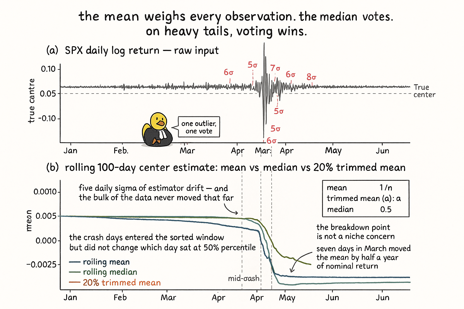
The two-panel diagnostic makes the breakdown-point argument concrete. The raw input has seven crash-week spikes; the rolling mean inhales them at weight 1/100 and drifts five daily-sigma off the bulk's actual center, while the rolling median ignores them by construction. The 20% trimmed mean is the intermediate option for cases where the median is too aggressive.

What this changes in practice

Three operational shifts.

Centering statistics in the feature library default to median, not mean. The feature definition stores the median and the IQR (or MAD) of the training window. The mean is computed and reported alongside for diagnostic purposes but is not used in the transform.

Smoothing primitives default to rolling median for outlier-prone series (volume, true range, absolute return) and rolling mean for bounded-by-construction series (RSI, Stochastic K). The default is recorded in the feature definition, not chosen at modeling time. Switching from rolling mean to rolling median on a known-outlier-prone primitive is a feature-design correction, not a modeling decision.

Correlation features in the feature library default to Spearman rank correlation, not Pearson. The Pearson correlation is computed and stored for diagnostic comparison. A feature whose Spearman and Pearson correlations differ by more than 0.10 over the same window is flagged for outlier inspection; the difference usually traces to one or two joint-tail observations that Pearson absorbed and Spearman did not.

KEY POINTS

• The mean has breakdown point 1/n. A single outlier can drive the mean to any value. The median has breakdown 0.5. Half the observations must be corrupted to move the median by more than a fixed amount.
• On heavy-tailed distributions (kurtosis 9 or higher), the median is more statistically efficient than the mean, not less. The "64% efficiency" Gaussian penalty does not apply to market data.
• Centering for sigmoid prep and forced centering: use the training-sample median. The training-sample mean is contaminated by the same tails the transform is being applied to remove.
• Spread measurement for variance scaling: use MAD or IQR. Standard deviation is dragged up by the tails and overestimates the bulk's spread. IQR ≈ 1.35 × MAD for Gaussian; both are L1-style robust alternatives.
• Smoothing for outlier-prone primitives (volume, true range, absolute return): use a rolling median filter. The moving average carries spikes at weight 1/W for W bars; the rolling median kills the spike as soon as it exits the sorted middle.
• Rolling median filters preserve edges (step changes). Moving averages round the corners of step changes over W bars. For primitives with mixed spike-and-step behavior, the median is the right filter.
• Correlation on heavy-tailed pairs: use Spearman or Kendall, not Pearson. Pearson can swing by 0.4 from a single joint-tail observation. Spearman moves at most 2/n per pair swap.
• Rolling-regression-based indicators (detrended RSI, deviation-from-prediction features): fit with LAD or Huber regression instead of OLS. OLS slopes are pushed by single outlier pairs; LAD and Huber slopes are stable.
• Use the mean when the distribution is light-tailed (RSI, Stochastic K), when the downstream computation requires an additive interpretation (portfolio P&L, total variance), or when the loss function is MSE.
• On SPX 100-bar rolling center, the mean spikes by 5 daily-σ through March 2020 and the median moves by 0.4 daily-σ. The mean is reporting the contamination; the median is reporting the bulk's center.
• The 20% trimmed mean is a hybrid that is more efficient than the median on moderately heavy-tailed data and less fragile than the mean. It is a reasonable default when the median is too aggressive and the mean is too fragile.
• The feature library defaults: centering = median, smoothing of outlier-prone primitives = rolling median, correlation = Spearman, robust regression = LAD or Huber. The mean is computed alongside for diagnostic comparison but is not the operational statistic.