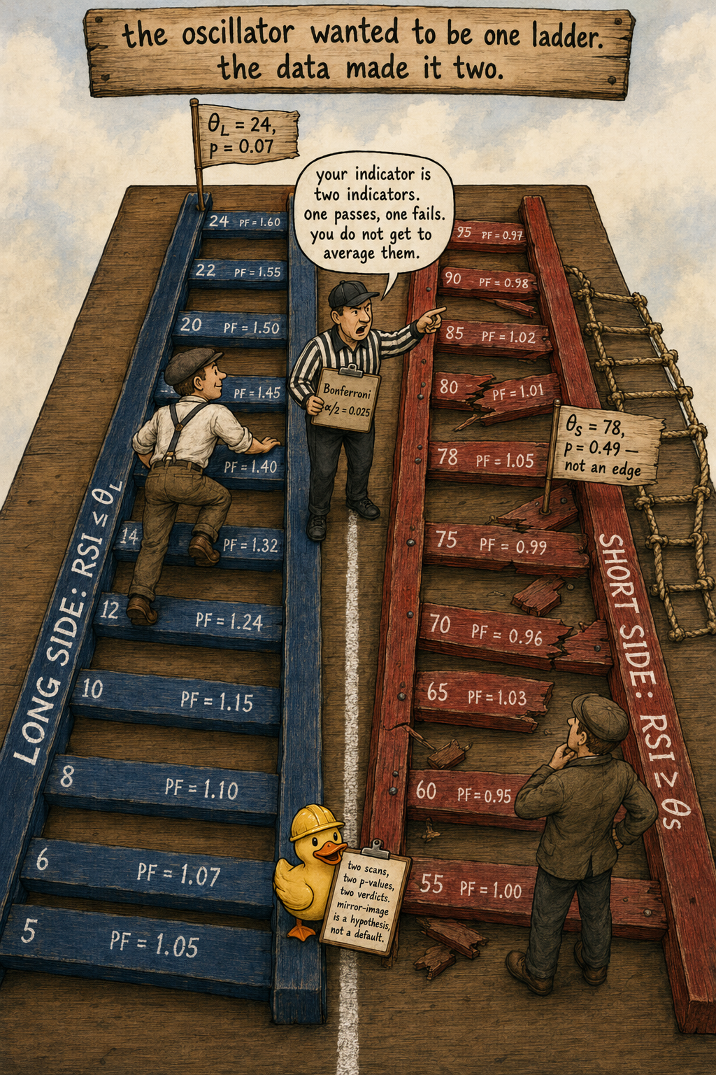
You take 14-day RSI on SPX and run the permutation-corrected threshold search from the article "How to Test Indicator Thresholds Without Fooling Yourself". The long side ("buy when RSI below θ_L") returns θ_L = 24 with permutation p = 0.07. The short side ("sell when RSI above θ_S") returns θ_S = 78 with permutation p = 0.49. You combine them into a single oscillator strategy with a 24/78 channel and report a portfolio Sharpe of 0.71.

Live, the long leg roughly tracks its backtest. The short leg loses money in a straight line for 14 months. The "Sharpe 0.71" you reported was a long-side edge contaminated by a short-side that was permutation-rejected before you bolted it on.

The mistake is structural. You treated the indicator as one object with one threshold scan, when the data is telling you it is two indicators with two scans and two null hypotheses. The long-side signal and the short-side signal live on different parts of the distribution, on different subpopulations, against different drifts. They have to be tested separately, reported separately, and accepted or rejected separately.

Why long and short are not mirror images

Four structural reasons, none of them controversial once stated.

Equities drift up. SPX has a roughly 7% annualized real drift and a positive daily mean. Any long-side rule inherits part of that drift as free baseline return. Any short-side rule has to swim against it. The same statistical edge produces different long-PF and short-PF numbers because the underlying unconditional means are different.

Return distributions are skewed. Equity daily returns have negative skew and fat left tails. A short-side rule that triggers in volatile regimes is selecting from a wider, fatter-tailed conditional distribution than the long-side mirror. The variance of the short-PF estimator is larger than the variance of the long-PF estimator at equal sample size.

Indicator distributions are asymmetric in their predictive content. The article "Why Predictive Power Often Lives in the Tails" showed that signal concentrates in extreme deciles. The signal in the upper decile and the signal in the lower decile are independent samples. RSI above 80 is overbought-regime conditional. RSI below 20 is panic-regime conditional. Two different market states with two different forward dynamics. Symmetry of the indicator construction does not imply symmetry of the predictive surface.

Selection bias doubles when you scan both sides. The permutation test in the prior article corrected for K candidate thresholds in one direction. If you scan K_L long thresholds and K_S short thresholds and report the best of either, your effective family-wise error rate is governed by K_L + K_S, not by K_L alone. The naive permutation that fixes a direction first does not correct for the cross-side selection.

The combined-test trap

A common framing: "the indicator carries information if either the long or the short threshold passes." This is true, and it is also the entry point for the bias.

Two protocols that look similar produce different results:

Protocol A. Test the long side at level α. Test the short side at level α. Report both p-values. Use long if its p passes α, use short if its p passes α, use both if both pass, use neither if neither pass.

Protocol B. Test both sides at level α. Report the better one. Apply no correction.

Protocol B is the one that produces the "Sharpe 0.71" headline. The family-wise error rate of Protocol B is approximately 2α minus the dependence-corrected overlap, which for nearly-independent long and short signals on a single indicator runs around 1.7α to 1.9α. A nominal 5% test reports false positives at 9% under Protocol B. The remedy is Bonferroni across the two sides, which works because the directional partition is exactly two and the conservatism cost is small. Run each side at α/2 = 0.025, or report the worse-side-adjusted p.

The harder failure is Protocol C, the silent one. The researcher computes long-side p and short-side p, looks at both, and writes the paper around whichever side passed. The reader sees one test. The selection across two has already happened.

Worked example: SPX 14-day RSI, two scans, two stories

SPX daily, 1990 to 2026, 9100 bars. Target y_t = sign(P_{t+1}/P_t - 1). Indicator: 14-day RSI.

Long-side scan: 41 candidate thresholds θ_L from 5 to 45 in steps of 1. Statistic: mean forward log return conditional on RSI ≤ θ_L versus unconditional mean.

Short-side scan: 41 candidate thresholds θ_S from 55 to 95 in steps of 1. Statistic: mean forward log return conditional on RSI ≥ θ_S versus unconditional mean, sign-flipped (short profit is positive when forward return is negative).

Five readings.

The long side has a borderline edge. Permutation-corrected p = 0.07 is above α = 0.05 but in the zone where a forward-window walk-forward (covered in the prior article) can confirm or reject. The structural story is consistent: RSI ≤ 24 on SPX selects panic-flush days that mean-revert. The sample size at this threshold is around 410 bars out of 9100.

The short side has no edge. Permutation-corrected p = 0.49 is consistent with pure chance. The structural story is also consistent: RSI ≥ 78 on SPX selects strong-trend days, and on an instrument with a 7% drift, those days continue more often than they reverse. The indicator's "overbought" reading is not a reversal signal on a trending instrument. It is a continuation signal disguised as a reversal by analogy to the long side.

The symmetric combined scan is the worst of three worlds. It assumes θ_L = 50 − δ and θ_S = 50 + δ for a single δ, which is the mirror-image constraint. The permutation p of the constrained scan is 0.21, which is above α. The constraint forced a fit to a symmetric model the data does not support. A single δ ≈ 26 splits the difference between a real long edge at δ_L = 26 and a non-edge short side at δ_S = 22, which is not where the short side's permutation maximum landed. The constraint averages a signal and a non-signal into a permutation-rejected blob.

Bonferroni at α = 0.05 across two sides demands each side's permutation p be below 0.025. Long fails at 0.07, short fails at 0.49. The honest verdict on the combined two-sided test is reject.

The single-side verdict on the long side at α = 0.05 is borderline-reject. The single-side verdict on the short side at α = 0.05 is reject. The bundled "Sharpe 0.71" oscillator is built on a borderline long edge plus a confirmed non-edge plus a symmetry assumption the data rejects.

The mirror-image fallacy in indicator design

A common construction: an oscillator centered at zero or fifty, with the rule "long when below −c, short when above +c, flat in between." The construction implies the predictive surface is anti-symmetric: whatever the indicator says about the long side at −c, it says the opposite for the short side at +c.

Three reasons the construction breaks on real data.

The base rate is not zero. Equities have positive drift. Currencies have positive interest carry on one leg. Commodities have term-structure roll. The neutral state of the rule is not "no position," it is "exposed to the baseline drift." A symmetric oscillator that closes positions in the middle subtracts the baseline drift it could otherwise harvest.

The conditional distributions on the two sides are not mirror images. RSI ≤ 24 selects high-volatility, large-negative-recent-return days. RSI ≥ 76 selects moderate-volatility, large-positive-recent-return days. The two subsamples have different volatilities, different higher moments, and different forward-window dynamics. The mean and the variance of the forward return inside each subsample are not related by a sign flip.

The thresholds that maximize each side's edge are not symmetric around the indicator's center. Long-side optima on equity indices typically sit deep in the lower tail (RSI 20 to 30). Short-side optima, when they exist, typically sit shallower (RSI 65 to 75) or at much deeper levels (RSI above 90) corresponding to blow-off tops rather than ordinary overbought regimes. Forcing θ_S = 100 − θ_L throws away both the optimal short threshold and the information that the optimal short threshold may not exist.

The right construction is two indicators glued together: I_long(t) = 1{X_t ≤ θ_L} with one threshold, and I_short(t) = 1{X_t ≥ θ_S} with a separately optimized and separately tested threshold. The two indicators share a common signal X but have independent thresholds, independent permutation tests, and independent walk-forward windows.

The asymmetric null

The block-bootstrap permutation from the prior article has to be run twice, once per side, with the same shuffled targets. Procedure:

1. Compute the long-side maximum t-statistic across K_L candidate thresholds on the real data. Record t_obs,L and θ_obs,L.
2. Compute the short-side maximum t-statistic across K_S candidate thresholds on the real data. Record t_obs,S and θ_obs,S.
3. Block-bootstrap the target series y with block length L (10 days for daily data).
4. On the shuffled (X, y_b), re-run both the long-side scan and the short-side scan. Record t_max,L,b and t_max,S,b.
5. Repeat for B = 5000 replications.
6. Compute p_L = (1/B) Σ_b 1{t_max,L,b ≥ t_obs,L} and p_S = (1/B) Σ_b 1{t_max,S,b ≥ t_obs,S}.
7. Two-sided Bonferroni decision: accept side d if p_d ≤ α/2. Accept the indicator if either side passes.

Three properties of this protocol matter.

The same shuffled targets are reused across the two sides per replication. The dependence between p_L and p_S under H_0 is preserved, so the joint distribution is correct rather than reconstructed from two independent runs.

Each side carries its own t_obs. The two p-values are not comparable in magnitude. A p_L of 0.07 and a p_S of 0.49 are two separate verdicts, not a single "p = 0.28 on average." Averaging would erase the directional information.

Bonferroni across two sides is small loss. The α/2 cut at 0.025 is 64% of the power of the α cut at 0.05 for a t-distribution. The cost of the correction is one-third of the power. The cost of skipping the correction is a doubled false-discovery rate on every two-sided indicator in your research portfolio.

The Long PF and Short PF table

Masters' framing computes the profit factor on each side at every candidate threshold, with the position held while the indicator satisfies the threshold and the win/loss tallied per bar (not per trade, which would artificially inflate the PF on consecutive same-direction bars).

The Long PF at threshold θ_L is sum of positive forward log returns conditional on X ≤ θ_L divided by sum of absolute negative forward log returns under the same condition. The Short PF at θ_S is the same calculation with the sign of the forward return flipped and the condition X ≥ θ_S. Plot both as functions of the cumulative fraction of bars selected.

The interpretive read of the plot is the one that survives outside the backtest.

A long-PF curve that rises smoothly as the threshold tightens (smaller selected fraction) is what the long-side edge looks like when it exists. The PF growth as the selection gets stricter is the tail-concentration result from "Why Predictive Power Often Lives in the Tails" expressed in PF units.

A short-PF curve that hovers near 1.0 across the threshold range, or that rises in the moderate threshold range and falls back at extreme thresholds, is what a non-edge looks like. The "rises in the middle" shape is the optimizer locating noise; the lack of consistency outside the middle is the data telling you the short-side signal is not structural.

A short-PF curve that rises only at the deepest tail (RSI above 90, for instance) is a separate signal from any moderate-overbought rule. The deep tail picks up blow-off tops. Treat it as its own indicator with its own threshold and its own permutation test.

Visualizing the asymmetry

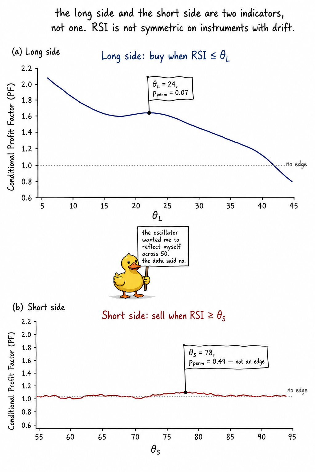
The two panels are the central diagnostic. One indicator construction, two scans, two completely different verdicts.

What this changes in practice

Three operational shifts.

Every directional indicator is tested as two indicators. Long-side scan and short-side scan are run independently against the same shuffled targets in a single permutation harness. Each side gets its own p-value, its own threshold, its own plateau check, and its own walk-forward. The combined "Sharpe of the bundled strategy" is reported only after both sides have independently passed their tests. If only one side passes, only that side ships, and the other side is documented as rejected, not silently dropped.

Symmetric thresholds are not assumed. The constraint θ_S = 100 − θ_L is a hypothesis to be tested, not a default. The two-sided permutation harness emits θ_L and θ_S as independent quantities. If the structural distance between them disagrees with the symmetric prior by more than a few percent of the indicator's range, the symmetric construction is rejected and the two thresholds are stored as two distinct numbers in the indicator-threshold registry.

Bonferroni at α/2 is applied across the two sides by default. The 33% power loss is the price for the doubled selection. Reporting only the better side without correction is the silent version of the bias and is treated as a research-process failure regardless of the underlying signal quality.

KEY POINTS

• The long-side threshold scan and the short-side threshold scan are two separate hypotheses on the same indicator. Equity drift, return skew, and conditional-distribution asymmetry make them statistically and structurally non-mirror.
• Equities have positive drift. Long-side rules harvest a fraction of that drift as baseline. Short-side rules fight it. Equal underlying edge produces different long-PF and short-PF numbers.
• Return distributions are negatively skewed on equity indices. Short-side conditional distributions are wider and fatter-tailed. The variance of the short-PF estimator exceeds the variance of the long-PF estimator at equal sample size.
• Scanning K_L long thresholds and K_S short thresholds and reporting the better is a selection across K_L + K_S, not across K_L. The naive single-direction permutation correction undercounts the family-wise error.
• The two-sided permutation harness runs both scans against the same block-bootstrap shuffled targets in each replication. The shared targets preserve the dependence between long and short null distributions.
• Bonferroni at α/2 across the two sides is the default correction. The 33% power loss is small relative to the doubled false-discovery rate of the uncorrected protocol.
• Symmetric thresholds (θ_S = C − θ_L for some center C) are a hypothesis, not a default. The two-sided scan emits independent θ_L and θ_S. Mirror-image is tested against the data, not assumed.
• Long-side optima on equity indices typically sit in the lower tail of RSI-style oscillators (20 to 30). Short-side optima, when they exist, either sit shallower or much deeper (above 90). Forcing symmetry erases both possibilities.
• A short-PF curve that hovers near 1.0 across the threshold range with a small bump in the middle is a non-edge. The bump is the optimizer locating the noise peak. The structural reading is no signal, regardless of the local maximum's nominal p.
• The bundled strategy Sharpe is reported only after both sides have independently passed their permutation tests. If only one side passes, only that side ships. The rejected side is documented, not silently bundled.
• On SPX 14-day RSI from 1990 to 2026, the long-side permutation p is 0.07 and the short-side permutation p is 0.49. The honest two-sided verdict at α = 0.05 with Bonferroni is reject. Some long-only deployments may still be defended at α = 0.10 with a walk-forward confirmation. No two-sided RSI oscillator on SPX survives the protocol.