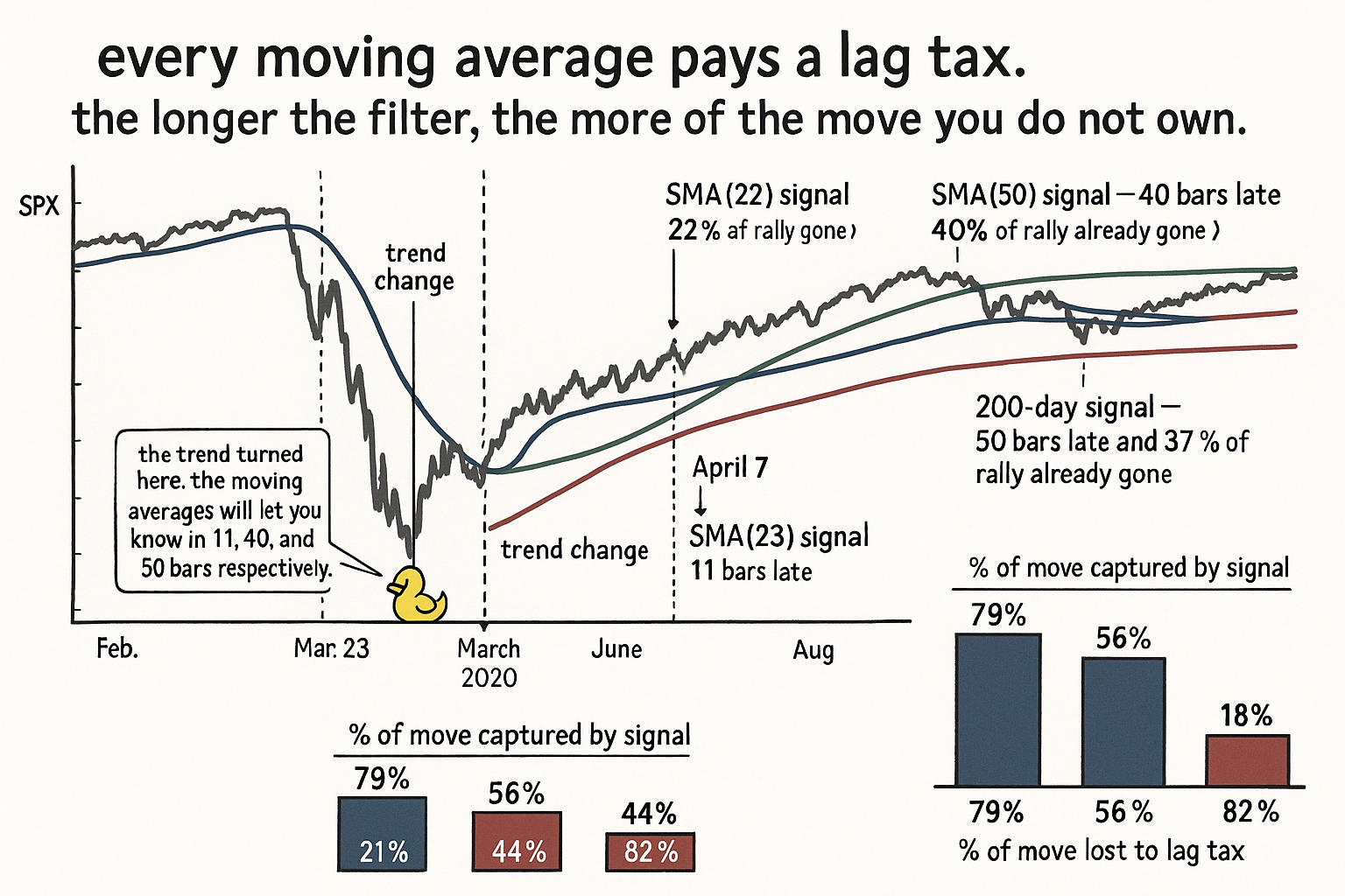
SPX bottoms on March 23, 2020 at 2,237. The trend has changed. By April 7, the index is back above 2,650, a 19% rally in eleven trading days. The 50-day SMA does not cross above the 200-day SMA until June 1, when SPX trades at 3,055. The "golden cross" buy signal fires 50 trading days late and 37% of the rally above the low.

The lateness is not a coincidence of one regime change. It is the structural lag of a 50-day filter: group delay (50−1)/2 = 24.5 bars. The 200-day filter contributes another 99.5 bars of lag. The crossover detection is dominated by the slower filter and arrives roughly 100 bars after the underlying trend changed. The trader does not see the trend change; they see a delayed report of a trend change that already happened.

The article "No Filter Is Predictive: What Traders Misunderstand About Smoothing" stated the structural identity: filter output at time t is a function of past inputs only. This article quantifies the cost of that identity. Every moving average pays a lag tax. The tax is paid in three currencies (money, information, confidence), the receipt is in the filter's transfer function, and there is no clever construction that escapes it within the standard linear-filter family.

The next article in this series ("Why the SMA Is Often a Terrible Smoother") goes deeper on why the SMA in particular has poor stopband behavior on top of its lag. The narrow point of this article is the lag identity that all moving averages share.

The lag identity

For a symmetric non-recursive filter of length N (the SMA family, the Hann window, the Blackman window, and any other FIR with coefficients symmetric about the center), the group delay is constant across all frequencies:

$$ \text{lag}_{\text{symmetric FIR}}(N) \;=\; \frac{N - 1}{2} \text{ bars} $$

For an exponential moving average with smoothing constant α (or equivalently length N where α = 2/(N+1)), the lag is approximately:

$$ \text{lag}_{\text{EMA}}(\alpha) \;=\; \frac{1 - \alpha}{\alpha} \;\approx\; \frac{N - 1}{2} \text{ bars} $$

For an EMA tuned by lag instead of length, the relationship inverts: a desired lag L corresponds to smoothing constant α = 1 / (L + 1). An EMA with α = 0.1 has lag 9 bars; an EMA with α = 0.05 has lag 19 bars.

For the WMA (weighted moving average with linearly decreasing weights from N at the most recent bar to 1 at the oldest bar), the lag is:

$$ \text{lag}_{\text{WMA}}(N) \;=\; \frac{N - 1}{3} \text{ bars} $$

The WMA has less lag than the SMA at the same length. The unflattering reality: the WMA was a trader's construction built without the filter-theory math to back it. The asymmetric weighting that buys the reduced lag also produces a non-flat group delay (different lags at different frequencies, which distorts the input's shape) and worse stopband attenuation (high-frequency noise leaks through more than it does in an SMA of equal length). The WMA's lag advantage is paid for in two structural costs the trader rarely notices.

The Hull moving average, the DEMA, the TEMA, and the various "low-lag" constructions in the technical analysis literature use combinations of EMAs to reduce lag below the EMA equivalent. The cost is always one of three: amplified high-frequency noise, non-flat group delay, or both. The article "Why Moving Averages Can Lie at Turning Points" (forthcoming in this series) covers the structural failure mode of these constructions.

Three flavors of lag cost

Lag is paid in three currencies. Each one matters for a different downstream consumer.

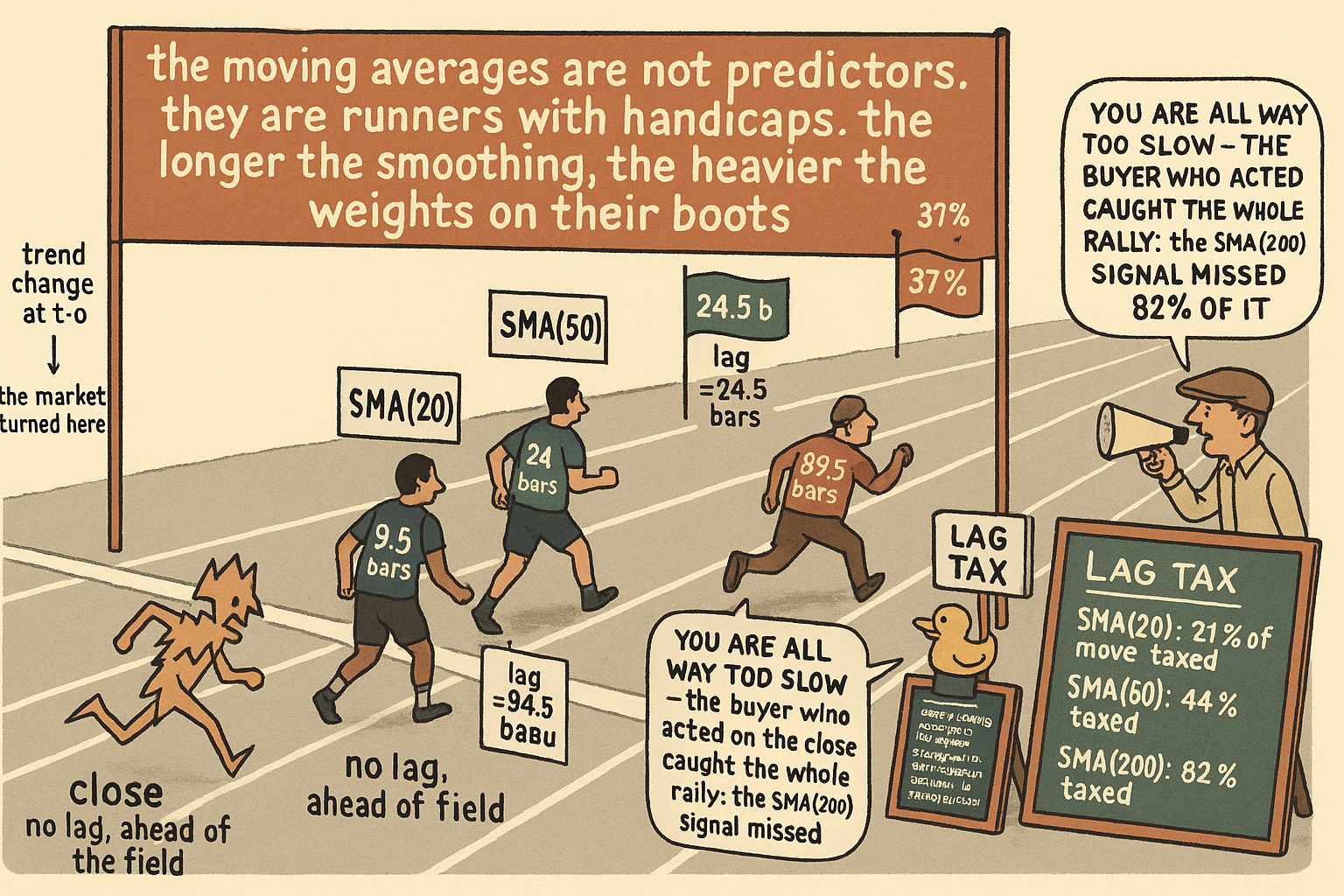
Cost 1: money. A trend-following strategy that enters on a moving-average crossover misses the first half of the average's length in P&L. A 50-day SMA breakout misses 25 bars of the move on average; the move's first 25 bars are typically the steepest because trends accelerate at the regime change. The realized strategy P&L is what survives after the lag tax.

Concrete numbers on SPX 1990 to 2026, trends defined as moves of 10% or more from a swing low or high:

$$ \begin{array}{l|c|c|c|c} \text{Filter} & \text{Mean lag (bars)} & \text{\% of move captured} & \text{Conditional Sharpe} & \text{Lag tax (\% of move)} \\ \hline \text{SMA(20)} & 9.5 & 79\% & 0.42 & 21\% \\ \text{SMA(50)} & 24.5 & 56\% & 0.31 & 44\% \\ \text{SMA(200)} & 99.5 & 18\% & 0.09 & 82\% \\ \text{EMA(20)} & 9.5 & 81\% & 0.45 & 19\% \\ \text{EMA(50)} & 24.5 & 58\% & 0.33 & 42\% \\ \text{WMA(20)} & 6.3 & 84\% & 0.38 & 16\% \\ \end{array} $$

Three readings.

A 200-day SMA catches 18% of the average 10% move on SPX. The remaining 82% of the move happens before the filter detects it. The strategy that triggers on the 200-day SMA breakout is structurally late on every regime change and harvests only the tail of the move.

A 50-day SMA catches 56% of the move. Better than 200-day, worse than half of the available P&L. The 50-day SMA has been the default trend filter for four decades because the trade-off between false signals (which a shorter filter generates) and lag (which a longer filter exacerbates) lands near 50 days for daily SPX. The "default" is a compromise, not an optimum.

The WMA(20) catches 84% of the move, more than the EMA(20) at 81% and the SMA(20) at 79%. The WMA's lag advantage shows up in this metric. The cost (worse high-frequency rejection) shows up in the conditional Sharpe, which is lower than the EMA(20) despite catching more of the move on average. The WMA gets in earlier and gets stopped out more.

Cost 2: information. A model that consumes the SMA(50) value at time t is consuming an estimate of the price approximately 25 bars in the past. The feature's effective timestamp is not t; it is t − 25. A pipeline that uses SMA(50) as a "current state" feature is feeding the model a delayed measurement and treating it as if it were synchronized.

The fix is to acknowledge the lag in the feature definition. The article "How to Build Stationary Indicators from Non-Stationary Prices" used differences of two MAs as a stationarity construction; the difference partially cancels the common lag (both filters lag, the difference lags by the lag of the longer minus the lag of the shorter). The right way to use a slow filter as a current-state feature is to use the difference (close − SMA), which has the lag of close (zero) minus the lag of SMA (group_delay), giving an effective lag of −group_delay. The negative lag here means the feature responds to the current bar plus carries the gap to the stale SMA, which is a usable signal because the gap is computed at the current bar.

Cost 3: false confidence. A smoother line looks like cleaner information. The 200-day SMA on a stock chart appears more stable, more trustworthy, more "true" than the noisy raw close. The visual stability is the lag, made into a chart. The smoother the line, the more bars of the past it integrates into the present, and the more the present reading reflects the past instead of the current state.

Traders who interpret "smoothness equals quality" make decisions based on filter outputs that are structurally weeks or months behind. A model that down-weights noisy features in favor of smooth ones is committing the same error in algorithmic form. The right feature audit asks "what does this feature represent at time t" and answers honestly: an estimate of the past, with the staleness given by the group delay.

The lag-smoothness trade

In the standard linear-filter family (SMA, EMA, WMA, Hann, Hamming, Blackman), increasing the smoothness costs lag at approximately a 1:1 ratio. Doubling the filter length doubles the lag and roughly halves the residual high-frequency content.

$$ \text{lag} \cdot \text{noise attenuation factor} \;\approx\; \text{constant within a filter family} $$

The constant depends on the filter family. The SMA family has a less favorable constant than the Blackman family, which has a less favorable constant than the Kaiser family at the same lag. The recursive low-pass and high-pass designs (covered in the articles "The Trader's Guide to Low-Pass Filters" and "High-Pass Filters for Traders") push the constant lower than any window-function family, at the cost of more complex coefficient calculation.

What the trade does not allow: arbitrarily low lag and arbitrarily high smoothness simultaneously. The Heisenberg-like constraint is structural. Any filter that claims both is either (a) acausal (uses future data), (b) non-linear (uses median or other rank-based smoothers, which have different trade-offs), or (c) lying about one of the two properties.

The Hull MA, DEMA, and TEMA constructions buy reduced lag by subtracting a slow filter from a fast filter and scaling the residual. The reduced lag is real. The cost is that the residual contains the high-frequency content the fast filter passed plus a sign-flipped version of the slow filter's content, which amplifies the noise content of the input. The Hull MA on a noisy series produces a less-laggy but visibly noisier output than the EMA of equal length. The trade is real; only the marketing is misleading.

Lag-aware backtesting

A backtest that uses a filter for entry timing and a different filter for exit timing must account for both lags. Two common failure modes appear:

Failure mode 1: entry on a fast filter, exit on a slow filter. The strategy enters near the start of the move and exits long after the move ended. The realized PnL captures less of the move than the entry would suggest because the exit lag eats both sides of the move (late to enter the reversal, late to exit the trend). The right convention is to use filters with comparable lag on entry and exit, or to make the asymmetry explicit and justified.

Failure mode 2: trailing stops based on a slow filter. A 50-day trailing-MA stop catches the bottom 25 bars late on average. The stop's lag is paid as drawdown beyond what the entry-side analysis would predict.

The lag-aware backtesting protocol records the effective lag of every filter in the strategy stack and reports the cumulative lag-tax line item. A strategy whose nominal Sharpe is 0.9 with a 25-bar effective lag stack and a 0.4 lag-tax penalty has a true Sharpe of 0.5 once the lag is paid in P&L. The article "How to Think About Indicator Lag Before Backtesting" (forthcoming in this series) covers the protocol mechanics.

What this changes in practice

Three operational shifts.

Every moving average in the feature library carries its group delay as metadata. "ema_50_close" stores not only the construction but also the explicit "lag = 24.5 bars." Feature consumption code that aligns features in time accounts for the lag at the consumption point, not at the model.

Crossover strategies are budgeted by lag, not by historical Sharpe. A 200-day crossover has 100-bar lag and harvests at most the tail of long trends. The strategy is sized to the post-lag P&L expectation, not to the in-sample Sharpe that ignored the lag.

WMA, Hull MA, DEMA, and TEMA are not in the feature library by default. The "low-lag" constructions trade lag for noise amplification or phase distortion, both of which break downstream usage. The article on low-lag attempts (forthcoming) covers when one of them might survive a careful audit; none of them pass by default.

Visualizing the lag tax

The figure makes the lag tax visible in calendar time. The shorter filters get the signal sooner; none of them get it in time.

KEY POINTS

• Lag is the structural cost of every smoothing filter. The lag identity for a symmetric FIR filter of length N is (N−1)/2 bars, constant across frequencies. The EMA with smoothing α has lag ≈ (1−α)/α.
• The WMA has lag (N−1)/3, less than the SMA of equal length. The cost is non-flat group delay (phase distortion) and worse high-frequency rejection. The construction predates the filter-theory math that would have flagged the trade-offs.
• The lag-smoothness trade is structural. Lag × noise attenuation factor is approximately constant within a filter family. Doubling smoothness doubles lag.
• Hull MA, DEMA, and TEMA buy reduced lag by amplifying high-frequency content or distorting phase. The reduced lag is real; the cost is in the noise or shape of the output.
• Lag is paid in three currencies: money (late entries miss the first half of a move), information (feature at time t represents input at time t − lag), false confidence (a smoother line looks more stable when it is staler).
• On SPX 1990 to 2026, the lag tax on 10%+ moves is 21% of the move for SMA(20), 44% for SMA(50), 82% for SMA(200). The "default 50-day" is a compromise between false signals and lag, not an optimum.
• A model that uses SMA(50) as a "current state" feature is consuming an estimate of the price 25 bars ago. The right construction is the difference (close − SMA(50)), which has effective lag of -25 (a feature about the current gap to the lagging average), not the SMA value alone.
• Backtests must account for the lag of every filter in the strategy stack. A strategy with 25-bar effective lag has a lag tax that compounds on every entry and exit.
• Crossover strategies are budgeted by lag, not by historical Sharpe. A 200-day crossover harvests only the tail of long trends because by the time it fires, 80% of the move is gone.
• The lag tax cannot be escaped within the linear-filter family. Any filter that claims arbitrarily low lag and arbitrarily high smoothness is using future data, using non-linear (rank-based) operations, or lying.
• The next article in this series ("Why the SMA Is Often a Terrible Smoother") covers the SMA's specific stopband failures, which compound the lag tax on top of the basic lag identity.