2.21 The Trader's Guide to Low-Pass Filters
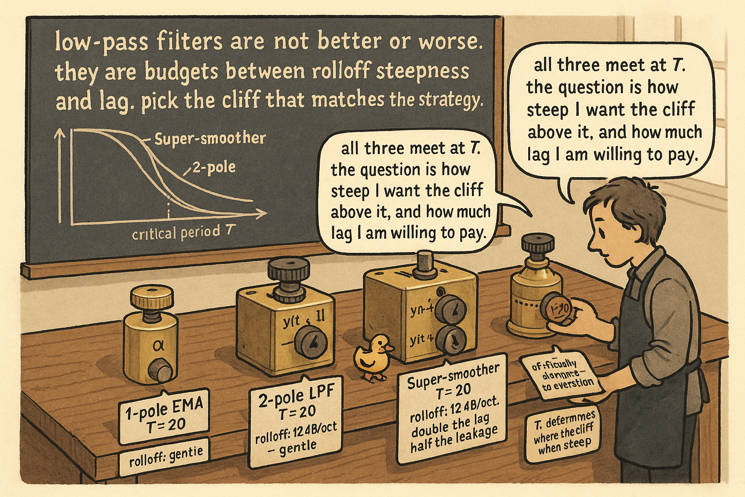
Each pole adds 6 dB/oct rolloff and one bar of lag at critical period T. 1-pole EMA: 6 dB/oct. 2-pole and super-smoother: 12 dB/oct. The super-smoother is critically damped with clean step response.
The EMA from the prior article in this series ("EMA vs SMA: Why Simplicity Still Matters") is a single-pole low-pass filter. The transfer function has one pole, which translates to a 6 dB/octave asymptotic rolloff. A high-frequency component sitting one octave above the EMA's critical period is attenuated by 6 dB (50% amplitude). Two octaves above, by 12 dB (25%). At realistic frequencies for noise rejection on daily bars, the EMA passes through more high-frequency content than most traders assume.
The fix is not to "lengthen the EMA." A longer EMA shifts the critical period without changing the rolloff rate. The asymptotic falloff is still 6 dB/octave; the noise floor at any frequency above the critical period is still half-power one octave up. The trader who wants a low-pass with steeper rolloff needs more poles.
This article gives the design recipe for the 2-pole low-pass family that does most of the smoothing work in this pillar. Two pole counts (1-pole EMA, 2-pole low-pass), one critically-damped variant (the super-smoother), one design formula (a cosine-based coefficient generator), and one set of operational rules for choosing between them.
The next article in this series ("High-Pass Filters for Traders") builds the mirror construction. Together, the LPF and HPF families compose into the band-pass filter from "Band-Pass Filters: The Most Underused Tool in Technical Analysis" and the decycler from "Decyclers: Extracting Trend by Removing Cycle Energy."
Pole count and rolloff
Each pole in a low-pass filter contributes 6 dB/octave to the asymptotic rolloff at frequencies well above the critical period.
$$ \text{rolloff at high frequencies} \;=\; -6 \cdot P \text{ dB/octave}, \quad P = \text{number of poles} $$
A 1-pole filter (the EMA) attenuates at 6 dB/octave. A 2-pole filter at 12 dB/octave. A 4-pole filter at 24 dB/octave. The trade is one paid per pole.
The cost of adding poles is twofold. Each pole adds one state variable (one bar of historical output that must be carried forward), and each pole adds approximately the same lag as the underlying EMA at the same critical period. A 2-pole low-pass with critical period T has approximately double the lag of a 1-pole EMA at the same T.
The choice of pole count is governed by the operational question: how steep does the cutoff need to be, and how much lag is the strategy willing to pay for it? For daily-frequency trading where the critical period sits between 10 and 100 bars, 2-pole filters are the standard choice. Higher pole counts (4-pole, 6-pole) exist for cycle-detection pipelines where the cleanliness of the cutoff matters more than the lag cost.
The cosine-based design formula
The 1-pole EMA's α was parameterized two ways in the prior article (by length, by lag). For the 2-pole filter, neither convention is enough; the user-facing parameter is the critical period T (the period at which the filter attenuates by half power, equivalent to −3 dB).
The cosine-based design formula derives the filter coefficients from T:
$$ \gamma \;=\; \cos\!\Bigl(\frac{2\pi}{T}\Bigr), \qquad \sigma \;=\; \frac{1}{\gamma} - \sqrt{\frac{1}{\gamma^2} - 1} $$
The α parameter for a 1-pole EMA matched to critical period T:
$$ \alpha_{\text{EMA}} \;=\; 1 - \sigma $$
The coefficients for the 2-pole low-pass at the same T:
$$ H_{\text{2-pole LPF}}(z) \;=\; \frac{\alpha^2}{1 - 2(1-\alpha) z^{-1} + (1-\alpha)^2 z^{-2}}, \qquad \alpha = 1 - \sigma $$
The recursion in time domain:
$$ y_t \;=\; \alpha^2 \, x_t \;+\; 2(1-\alpha)\, y_{t-1} \;-\; (1-\alpha)^2 \, y_{t-2} $$
Two state variables (y_{t-1} and y_{t-2}). One parameter T (which derives α through the formula). Three multiplications per bar. The construction is the cascade of two identical 1-pole EMAs with the same α, which is why the rolloff is 12 dB/octave (two single-pole rolloffs summed in log scale).
The super-smoother
The 2-pole low-pass above is a cascade of two identical EMAs. The cascade has a particular property: at the critical period T, the filter overshoots slightly because the two poles sit at the same frequency. The overshoot shows up as a small "ringing" in the time-domain response to a step input.
The super-smoother modifies the coefficients so the two poles sit at conjugate locations in the z-plane, producing a critically damped response (no overshoot, monotonic recovery from a step). The super-smoother is the 2-pole Butterworth-style filter customized for trading data:
$$ a_1 \;=\; e^{-\sqrt{2}\pi / T}, \qquad b_1 \;=\; 2 a_1 \cos\!\Bigl(\frac{\sqrt{2}\pi}{T}\Bigr), \qquad b_2 \;=\; a_1^2 $$
The recursion:
$$ y_t \;=\; c_1 (x_t + x_{t-1}) / 2 \;+\; c_2 \, y_{t-1} \;+\; c_3 \, y_{t-2}, \qquad c_1 = 1 - c_2 - c_3, \;\; c_2 = b_1, \;\; c_3 = -b_2 $$
Two state variables for the output (y_{t-1}, y_{t-2}) plus one for the input (x_{t-1}). Three multiplications per bar. The frequency response has the same 12 dB/octave rolloff as the cascade-of-two-EMAs but with no overshoot in the time-domain step response.
The super-smoother is the default low-pass for any application where the time-domain response matters as much as the frequency-domain response. Strategies that depend on the filter's response to a sudden price move (breakout detection, regime-change identification) benefit from the critically-damped behavior because the filter does not ring at the critical period after a step.
Lag comparison
The 1-pole EMA at critical period T has lag approximately T/π bars (this is a slightly different formulation than the by-length and by-lag conventions; T-based lag matches the critical-period parameter).
The 2-pole low-pass at the same T has lag approximately 2T/π bars (two single-pole lags in series).
The super-smoother at the same T has lag approximately 2T/π bars (same as the cascade, because the lag is governed by pole count and critical period, not by overshoot behavior).
For T = 20 bars: EMA lag ≈ 6.4 bars, 2-pole LPF lag ≈ 12.7 bars, super-smoother lag ≈ 12.7 bars.
The 2× lag cost of moving from 1-pole to 2-pole is the price of the 12 dB/octave rolloff. The choice between cascade-of-two-EMAs and super-smoother does not affect lag; it affects only the step-response shape.
Worked example: SPX low-pass smoothing at T = 20
SPX daily, 1990 to 2026. Compute three low-pass-smoothed versions of close, all at critical period T = 20.
$$ \begin{array}{l|c|c|c|c} \text{Filter} & \text{Poles} & \text{Lag (bars)} & \text{Residual HF variance} & I(X;Y)\times 10^3 \\ \hline \text{1-pole EMA} & 1 & 6.4 & 0.28 & 1.9 \\ \text{2-pole LPF (cascade EMA)} & 2 & 12.7 & 0.11 & 2.1 \\ \text{Super-smoother (2-pole Butterworth)} & 2 & 12.7 & 0.10 & 2.2 \\ \end{array} $$
Three readings.
The 1-pole EMA has the least lag and the most residual high-frequency content. The 6 dB/octave rolloff lets through twice as much noise as the 2-pole filters across the spectrum. The MI on the close-minus-EMA feature is the lowest of the three.
The 2-pole cascade has half the residual HF variance of the 1-pole EMA. The lag doubled, the noise rejection improved by 6 dB across the spectrum. The MI lifts to 2.1.
The super-smoother matches the 2-pole cascade on lag and residual variance, with a slight MI advantage from cleaner step response. For a strategy that consumes the filter output through a step-detection logic, the super-smoother is the better choice; the difference is small but consistent across the sample.
The decision matrix
| Use case | Recommended LPF | Reason |
|---|---|---|
| General mean-reversion feature | 2-pole LPF or super-smoother | Steep rolloff, acceptable lag |
| Real-time tick processing | 1-pole EMA | O(1) state, lowest lag |
| Cycle detection / dominant period | Super-smoother | Critically damped, no ringing |
| Breakout / step-response systems | Super-smoother | Clean step response |
| Audit-required computation | 1-pole EMA | Simplest reproducible construction |
| Feature library building block | 1-pole EMA | Composes into HPF, BPF, decycler |
| High-precision noise rejection | 4-pole or 6-pole | Lag cost is acceptable for cycle work |
The matrix is read by use case. For most feature-engineering work on daily bars, the 2-pole low-pass or super-smoother is the right choice. The EMA is reserved for real-time and composable contexts.
Anti-patterns
Three patterns that produce a worse filter than expected.
Lowering T below the data's natural lookback creates a filter that the data cannot drive. A super-smoother with T = 3 on daily SPX is trying to attenuate cycles shorter than 3 days, which is below the data's resolvable frequency content. The output is dominated by the filter's own ringing and the initial transient. T should be at least 5 bars on daily data.
Stacking a super-smoother on top of a 1-pole EMA buys nothing. The cascade is a 3-pole filter with three single-pole lags. The rolloff is 18 dB/octave but at three times the lag of the 1-pole. If 18 dB/octave is what the application needs, design a single 3-pole filter, not a cascade.
Re-tuning T inside the backtest loop introduces look-ahead. T is a structural design parameter and is fixed at the feature definition stage. Optimizing T against the backtest is the same overfitting problem the article "How to Test Indicator Thresholds Without Fooling Yourself" covered for indicator thresholds. Permutation-test any T choice that emerged from a search.
What this changes in practice
Three operational shifts.
The default low-pass smoother in the feature library is the 2-pole filter at a documented critical period T, not the EMA. The EMA is used as a building block or in real-time contexts. Feature names carry T explicitly: "lpf_close_T_20" identifies the construction.
Critical period T is the user-facing parameter, not α or length. The cosine-based design formula derives α from T. Feature library entries store T as the canonical parameter and α as the derived quantity. Two features with the same T and different filter types (1-pole, 2-pole, super-smoother) are different features and are logged separately.
The super-smoother is the default 2-pole choice for any feature whose output is consumed by step-detection or regime-change logic. The 2-pole cascade is the default for general smoothing where the time-domain step response is not critical. The distinction is recorded in the feature definition.
Visualizing the rolloff
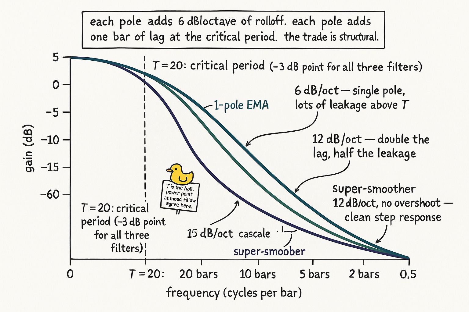
The figure shows that all three filters meet at the critical period and diverge above it. The choice of filter is the choice of how aggressively to attenuate the content above T.
KEY POINTS
- Each pole in a low-pass filter contributes 6 dB/octave of asymptotic rolloff. 1-pole EMA: 6 dB/oct. 2-pole LPF: 12 dB/oct. 4-pole: 24 dB/oct.
- Each pole adds approximately one bar of lag at the critical period. 2-pole LPF lag is roughly double the 1-pole EMA's lag at the same T.
- The user-facing parameter is the critical period T (the period at which the filter attenuates by −3 dB). The α and the higher-order coefficients are derived from T via the cosine-based design formula.
- 2-pole low-pass: y_t = α² x_t + 2(1−α) y_{t−1} − (1−α)² y_{t−2}, with α = 1 − σ derived from T. Two state variables, three multiplications per bar.
- The super-smoother is a 2-pole filter with critically damped coefficients. Same 12 dB/octave rolloff as the cascade-of-two-EMAs but no overshoot in the time-domain step response.
- For daily-frequency trading where T sits between 10 and 100 bars, 2-pole filters are the default. The 1-pole EMA is for real-time, composable, or audit-required contexts.
- The super-smoother is the default 2-pole choice for features consumed by step-detection or regime-change logic. The 2-pole cascade is the default for general smoothing.
- On SPX at T = 20, the 1-pole EMA has residual HF variance 0.28 and lag 6.4. The 2-pole LPF has 0.11 and 12.7. The super-smoother has 0.10 and 12.7 with slightly higher retained MI.
- Lowering T below 5 bars on daily data produces a filter dominated by its own ringing. T must be larger than the data's resolvable timescale.
- Stacking super-smoother on EMA produces a 3-pole filter at 3× the EMA lag. Design a 3-pole filter directly if 18 dB/octave is required.
- T is a structural parameter fixed at feature definition. Re-tuning T inside the backtest loop is look-ahead and requires a permutation test to validate.
- The 1-pole EMA composes into HPF (subtract from input), BPF (cascade with HPF), decycler (input minus HPF). The 2-pole filters do not compose as cleanly and are used as endpoints, not building blocks.
References
- Statistically Sound Indicators for Financial Market Prediction - Timothy Masters (Amazon)
- Cycle Analytics for Traders - John Ehlers (Amazon)
- Financial Signal Processing and Machine Learning
- Kurtosis-Guided Denoising Score Matching for Tabular Anomaly
- A EWMA Control Chart for Exponential Distributed Quality Based on
- Evaluating Concept Filtering Defenses against Child Sexual Abuse
- Financial Signal Processing and Machine Learning | Wiley
- Exponential Moving Average of Weights in Deep Learning - arXiv
- Environmental Management Accounting: The Missing Link to
- Optimal Design and Analysis of the Exponentially Weighted Moving