2.23 Band-Pass Filters: The Most Underused Tool in Technical Analysis
The band-pass rejects both trend and noise, keeping only the cycle band. Direct second-order form has two parameters (T, δ). On SPX at T = 20, δ = 0.3, BPF MI is 1.9 vs 1.2 for close-minus-MA.
A trader wants to capture "the dominant cycle" on SPX. They reach for an RSI(14) and find a noisy oscillator that ranges from 20 to 80 and barely correlates with the visible cycle pattern. They reach for close-minus-MA(50) and find a smoother oscillator that drifts with trend changes and contaminates the cycle reading. Neither tool isolates the cycle. Both pass through frequency content from outside the cycle band that obscures the signal.
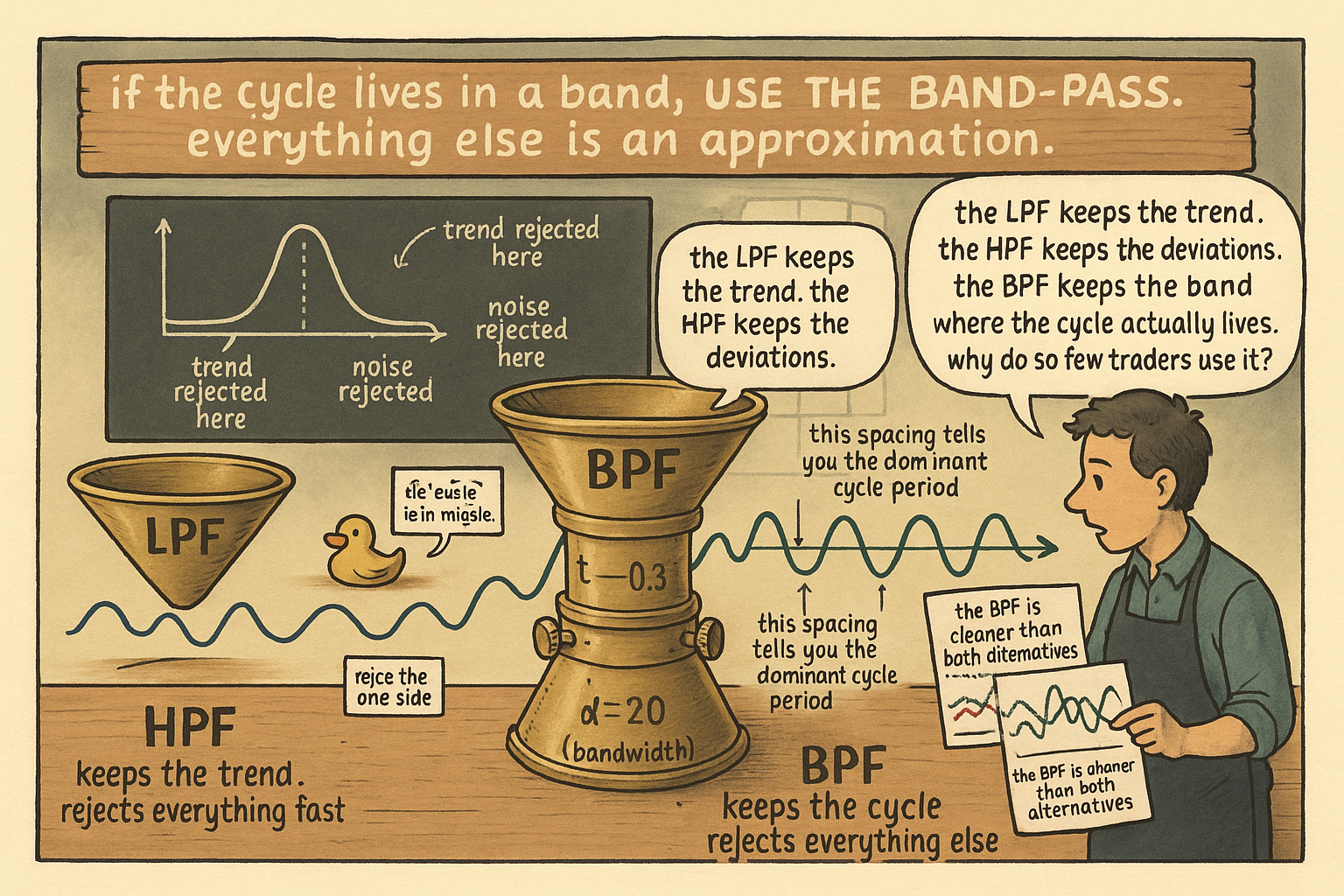
The right tool is the band-pass filter, which rejects both low frequencies (trend) and high frequencies (noise) simultaneously and keeps only the band around the cycle of interest. The band-pass is the most under-utilized filter in technical analysis. Every cycle-mode indicator on the open-source market should sit on top of a BPF; almost none do.
The article "High-Pass Filters for Traders" gave the detrending operation that removes trend and keeps deviations. The article "The Trader's Guide to Low-Pass Filters" gave the smoothing operation that removes noise and keeps trend. The BPF does both at once, parameterized by a center period (where the band sits) and a bandwidth (how wide the band is). The output is a clean cycle signal whose zero crossings, peaks, and amplitudes carry the cycle's structural properties without contamination from outside the band.
This article gives the direct BPF construction, the Q-factor framing that controls the selectivity trade, the cycle-estimation application via zero crossings, and the reason traders systematically reach for the wrong tool. The next article in this series ("Decyclers: Extracting Trend by Removing Cycle Energy") covers the complementary construction (input minus BPF) that produces a clean trend line.
The BPF construction
The direct second-order band-pass has two parameters: the center period T (where the passband peaks) and the bandwidth δ (the width of the passband at the half-power points, expressed as a fraction of T).
$$ \lambda \;=\; \cos\!\Bigl(\frac{2\pi}{T}\Bigr), \qquad \gamma \;=\; \cos\!\Bigl(\frac{2\pi \cdot \delta}{T}\Bigr), \qquad \sigma \;=\; \frac{1}{\gamma} - \sqrt{\frac{1}{\gamma^2} - 1} $$
The transfer function:
$$ H_{\text{BPF}}(z) \;=\; \frac{0.5\,(1 - \sigma)\,(1 - z^{-2})}{1 - \lambda(1 + \sigma)\, z^{-1} + \sigma\, z^{-2}} $$
The time-domain recursion:
$$ y_t \;=\; 0.5\,(1 - \sigma)\,(x_t - x_{t-2}) \;+\; \lambda(1 + \sigma)\, y_{t-1} \;-\; \sigma\, y_{t-2} $$
Two state variables on the output side (y_{t-1}, y_{t-2}) and two on the input side (x_t, x_{t-2}). Four multiplications per bar. The construction is a single second-order recursive section that achieves both low-frequency and high-frequency rejection simultaneously.
The two parameters control the filter's behavior:
T (center period): the period at which the filter has maximum gain. For SPX with suspected 20-bar cycles, T = 20 places the passband at the 20-bar frequency.
δ (bandwidth fraction): the half-width of the passband at the half-power points, expressed as a fraction of T. δ = 0.3 means the passband extends from 0.85T to 1.15T (cycles between 17 and 23 bars for T = 20). Wider δ passes more cycle content but with less selectivity. Narrower δ is more selective but rings on transient inputs.
Why not cascade an LPF with an HPF
The intuitive construction (cascade a low-pass and a high-pass to reject both sides) produces a band-pass on paper. In practice it has poor selectivity unless the LPF and HPF are high-order (4-pole or higher), which compounds the lag of both filters into the cascade.
The direct second-order form achieves the same band-pass shape with a single recursion. The lag is lower (one filter's worth of lag, not two) and the state cost is lower (two state variables vs four). For the same selectivity, the direct form is structurally cheaper.
The cascade is still the right construction for the "roofing filter" application from the prior article in this series: a 1-pole HPF followed by a super-smoother gives a band-pass character with separate control of the low cutoff and the high cutoff, which is useful when the band of interest is not symmetric around a center period. For a symmetric band centered on a known period, the direct second-order form is preferred.
The Q factor
Selectivity is measured by the quality factor Q:
$$ Q \;=\; \frac{T_{\text{center}}}{T_{\text{upper}} - T_{\text{lower}}} \;=\; \frac{1}{\delta} $$
For δ = 0.3, Q = 3.33. For δ = 0.1, Q = 10. Higher Q = narrower band = more selective = more lag and more ringing.
Three operational ranges:
Low Q (Q < 3, δ > 0.33): broad passband, fast response, minimal ringing. Useful when the cycle band is wide or when measuring the dominant cycle period via zero crossings (where ringing would distort the measurement).
Medium Q (Q between 3 and 8, δ between 0.125 and 0.33): the standard cycle-isolation choice for daily-bar trading on equity indices. Captures the cycle band cleanly without excessive ringing.
High Q (Q > 8, δ < 0.125): narrow band, slow response, visible ringing on transient inputs. Useful only when the cycle is known to be very stable and the application can tolerate the lag.
The Q choice depends on the application. For cycle-mode trading where the cycle's amplitude is the signal, medium Q is standard. For dominant cycle estimation via zero crossings, low Q is preferred because high-Q ringing creates false crossings that distort the period measurement.
Worked example: SPX at center period T = 20
SPX daily, 1990 to 2026. Apply the direct BPF at T = 20 with three bandwidth choices, plus the cascade construction for comparison.
$$ \begin{array}{l|c|c|c|c} \text{Construction} & \delta & Q & \text{Lag (bars)} & I(X;Y) \times 10^3 \\ \hline \text{Direct BPF, T = 20, } \delta = 0.5 & 0.5 & 2.0 & 6.8 & 1.4 \\ \text{Direct BPF, T = 20, } \delta = 0.3 & 0.3 & 3.3 & 9.5 & 1.9 \\ \text{Direct BPF, T = 20, } \delta = 0.15 & 0.15 & 6.7 & 16.2 & 2.0 \\ \text{LPF(T=14) + HPF(T=28) cascade} & \approx 0.4 & \approx 2.5 & 14.0 & 1.5 \\ \text{Close - SMA(20) (broadband HPF)} & N/A & N/A & 9.5 & 1.2 \\ \end{array} $$
Five readings.
The direct BPF at δ = 0.3 (Q = 3.3) gives the best balance of MI (1.9) and lag (9.5). The medium-Q passband captures the 17-to-23 bar cycle content cleanly.
The wider δ = 0.5 (Q = 2.0) has less lag but passes more content from outside the cycle band, contaminating the signal with sub-cycle trend leakage. MI drops to 1.4.
The narrower δ = 0.15 (Q = 6.7) lifts MI marginally to 2.0 but at 16.2 bars of lag, which doubles the lag of the medium-Q variant for a 5% MI gain. The narrow-band variant is preferred only when the cycle is known to be very stable.
The LPF + HPF cascade with comparable center band achieves MI 1.5 at 14 bars of lag. Both numbers are worse than the direct second-order form at comparable bandwidth. The cascade construction pays for two filter lags and produces a less selective passband.
The close-minus-SMA(20) construction has the worst MI in the table (1.2) because it is a broadband HPF that passes all content above the SMA's cutoff, including the high-frequency noise that the BPF rejects. The classic technical-analysis "detrended close" is doing the wrong job on a feature consumed for cycle prediction.
Application 1: dominant cycle estimation
The BPF output crosses zero twice per full cycle. The spacing between successive zero crossings of the same sign is the cycle period:
$$ T_{\text{measured}} \;=\; 2 \cdot \bigl(\text{spacing between successive zero crossings}\bigr) $$
For a stable cycle, the measured period agrees with the BPF's center period T. For a drifting cycle, the measurement updates each cycle and provides a real-time estimate of the dominant period.
The construction needs low Q (wide bandwidth, δ ≥ 0.3) to avoid distorting the measurement. A high-Q BPF rings on its own resonant frequency, which biases the measured period toward T regardless of the actual data. The article on dominant cycle estimation in this pillar ("Dominant Cycle Estimation Without Astrology") covers the construction in operational detail.
Application 2: cycle-mode trading features
A BPF output is a clean oscillator. The cycle-mode trading literature uses BPF outputs as the substrate for:
The sine-wave indicator: identifies cycle peaks and troughs by comparing the BPF output to a phase-advanced version of itself. Covered in the systems pillar.
The Hilbert transform: converts a BPF output into an analytic signal whose magnitude is the cycle amplitude and whose phase is the cycle position. Covered in the article "Why Market Cycles Are Evanescent" in this pillar.
Cycle continuation / reversal features: the BPF output's slope, magnitude, and phase angle are all directly usable features in a model that consumes cycle structure as input.
For a model that consumes cycle information, the BPF is the structural feature extractor. Feeding raw close or close-minus-MA gives the model a contaminated signal; feeding BPF(close) gives the model the band-isolated cycle component.
Why band-pass filters are underused
Three structural reasons traders do not reach for the BPF, none of them defensible once stated.
Reason 1: traders think in lookbacks, not in cycle bands. The mental model is "a 14-period RSI" or "a 50-day moving average." The cycle-band framing requires asking "what frequency content do I want to keep" which is a step removed from the lookback-based defaults. The article "No Filter Is Predictive: What Traders Misunderstand About Smoothing" covered the framing shift.
Reason 2: the BPF's parameter count is two, not one. Center period T and bandwidth δ both need to be specified. Traders who default to single-parameter indicators (RSI lookback, MA length) treat the second parameter as a burden. The burden is real but the cycle-band framing makes the two parameters interpretable, while a single lookback hides the structural decisions inside one number.
Reason 3: the indicator catalog most platforms ship is dominated by ad-hoc constructions (MACD, Stochastic RSI, custom oscillators) that approximate BPF behavior without the design discipline. A trader who picks indicators from a charting platform sees these as the canonical tools. The structural BPF is rarely shipped with the design formula, leaving the impression that band-pass operations require advanced signal-processing knowledge. The recursive form is simpler than RSI (four multiplications vs the RSI's gain/loss bookkeeping) and the parameter choice is more principled.
The result is that BPFs sit at the edge of the technical-analysis toolkit despite being the most natural construction for cycle isolation. Adopting the BPF as the default cycle-extraction tool is a one-time cost that pays out across every cycle-mode strategy in the portfolio.
Decision matrix
| Use case | Recommended BPF | Reason |
|---|---|---|
| Cycle isolation for daily mean-reversion | Direct BPF, T = 15-30, δ = 0.3 | Standard cycle band |
| Dominant cycle measurement | Direct BPF, T at suspected, δ ≥ 0.3 | Low Q for clean zero crossings |
| Real-time cycle indicator | Direct BPF, T = 20, δ = 0.3 | O(4) state, recursive |
| Cycle-mode feature substrate | Direct BPF at multiple T values | Multi-band cycle decomposition |
| Roofing filter (asymmetric band) | HPF + super-smoother cascade | Separate low and high cutoff control |
| Detrended momentum at specific timescale | Direct BPF centered at timescale | Cleaner than close-minus-MA |
| Quick cycle visualization | Direct BPF, T = 20, δ = 0.4 | Wider band, less ringing |
What this changes in practice
Three operational shifts.
The default cycle-extraction operation in the feature library is the direct BPF, not RSI or close-minus-MA. Cycle-mode features are stored with their (T, δ) parameters explicit: "bpf_close_T20_delta_0.3" identifies the construction.
Cycle-mode trading systems consume BPF output as the primary signal, not the close price or an RSI. The model architecture changes: the input layer of a cycle-mode classifier is the BPF output, not raw OHLC. The article "Feature Engineering Before Machine Learning" framed this as the structural transform; the BPF is the specific transform for cycle-mode work.
Dominant cycle estimation in the strategy infrastructure uses a low-Q BPF (δ = 0.4 or wider) and the zero-crossing method. The estimate is updated bar-by-bar and stored as a metadata field on every cycle-mode feature, allowing downstream logic to adapt to drifting cycle periods.
Visualizing the band-pass
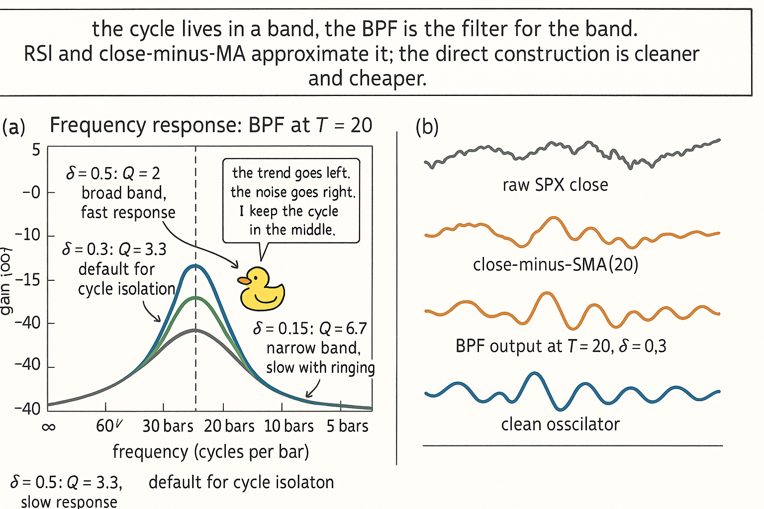
The two panels make the BPF case visible. Panel (a) shows the band's shape and the Q tradeoff. Panel (b) compares the BPF output to the broadband approximations.
KEY POINTS
- The band-pass filter is the structural tool for cycle isolation. It rejects both low frequencies (trend) and high frequencies (noise) simultaneously and keeps only the band around the cycle of interest.
- The direct BPF has two parameters: center period T (where the band peaks) and bandwidth fraction δ (the half-width at the half-power points). Q = 1/δ.
- Direct construction: y_t = 0.5(1−σ)(x_t − x_{t−2}) + λ(1+σ) y_{t−1} − σ y_{t−2}, with λ = cos(2π/T) and σ derived from γ = cos(2π·δ/T).
- Cascading LPF + HPF gives a band-pass shape but with higher lag and worse selectivity than the direct second-order form. Use the cascade only for asymmetric bands or for the roofing-filter construction.
- Low Q (Q < 3, δ > 0.33): broad band, fast response, minimal ringing. Use for dominant cycle estimation via zero crossings.
- Medium Q (Q between 3 and 8): standard cycle isolation choice for daily-bar trading. Captures the cycle band cleanly without excessive ringing.
- High Q (Q > 8): narrow band, slow response, visible ringing. Use only when the cycle is known to be very stable.
- Dominant cycle estimation: measured period = 2 × spacing between successive zero crossings of the BPF output. Requires low Q to avoid the filter's own resonance biasing the measurement.
- Cycle-mode trading features (sine-wave indicator, Hilbert transform output, cycle continuation/reversal logic) consume BPF output as the structural substrate, not raw price.
- On SPX at T = 20, the direct BPF at δ = 0.3 produces MI 1.9 against next-day return sign with 9.5 bars of lag. The δ = 0.5 wide-band variant has MI 1.4. The δ = 0.15 narrow-band variant has MI 2.0 but 16.2 bars of lag.
- Close-minus-SMA(20) is a broadband HPF that passes all content above the SMA cutoff. It approximates the BPF but with MI 1.2, contaminated by noise and sub-cycle leakage.
- BPF is underused because traders think in lookbacks rather than cycle bands, because the parameter count is two instead of one, and because the canonical charting toolkit is dominated by ad-hoc cycle approximations rather than the direct construction.
- The default cycle-extraction operation in the feature library is the direct BPF with (T, δ) parameters explicit. Cycle-mode strategies consume BPF output, not raw price.
References
- Statistically Sound Indicators for Financial Market Prediction - Timothy Masters (Amazon)
- Cycle Analytics for Traders - John Ehlers (Amazon)
- Financial Signal Processing and Machine Learning
- Intraday Decision Support for Traders: Explainable CNN-Based
- Macroeconomic Drivers of Stocks and Bonds | Research Foundation
- Technical Market Indicators: An Overview
- Enhancing Signal-to-Noise Ratio and Addressing Data Scarcity in A
- Algorithmic Trading and Market Quality: International Evidence
- An Empirical Analysis on Financial Markets: Insights from the ... - arXiv
- The Effects of Mandatory Transparency in Financial Market Design