2.28 Why Median Filters Are Useful for Volume and Outliers
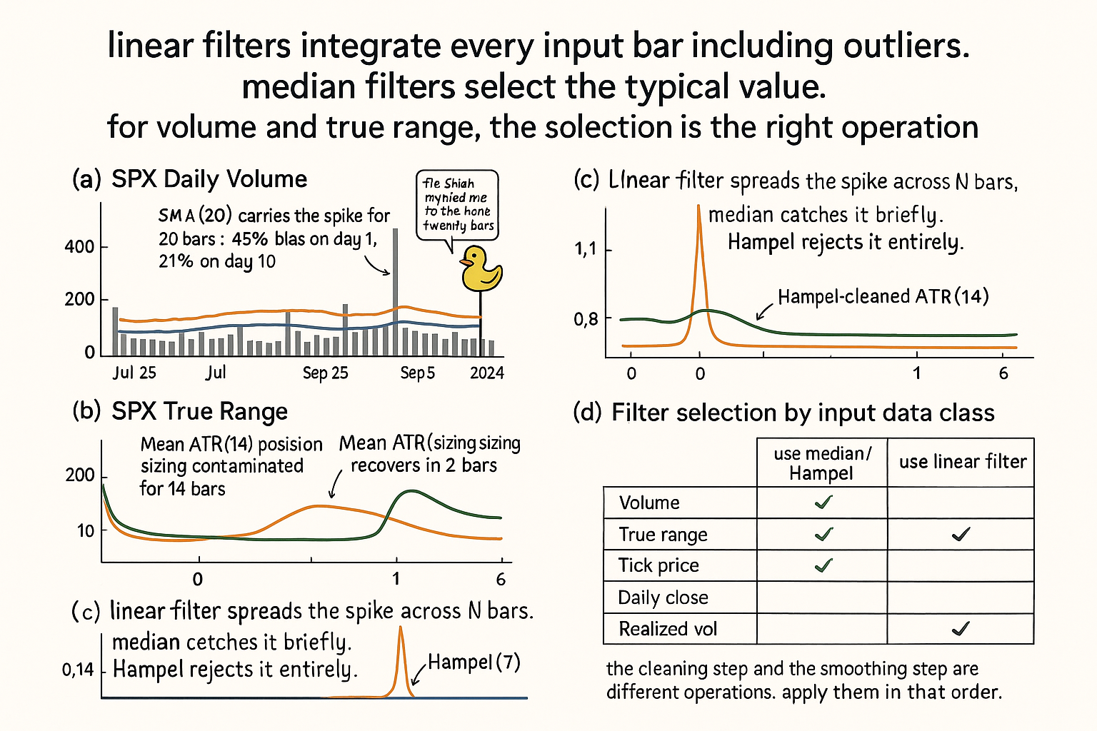
Linear filters integrate every bar including outliers. Median filters select the typical value. For volume, true range, and tick data, median (or Hampel) is the default; linear smoothers come after.
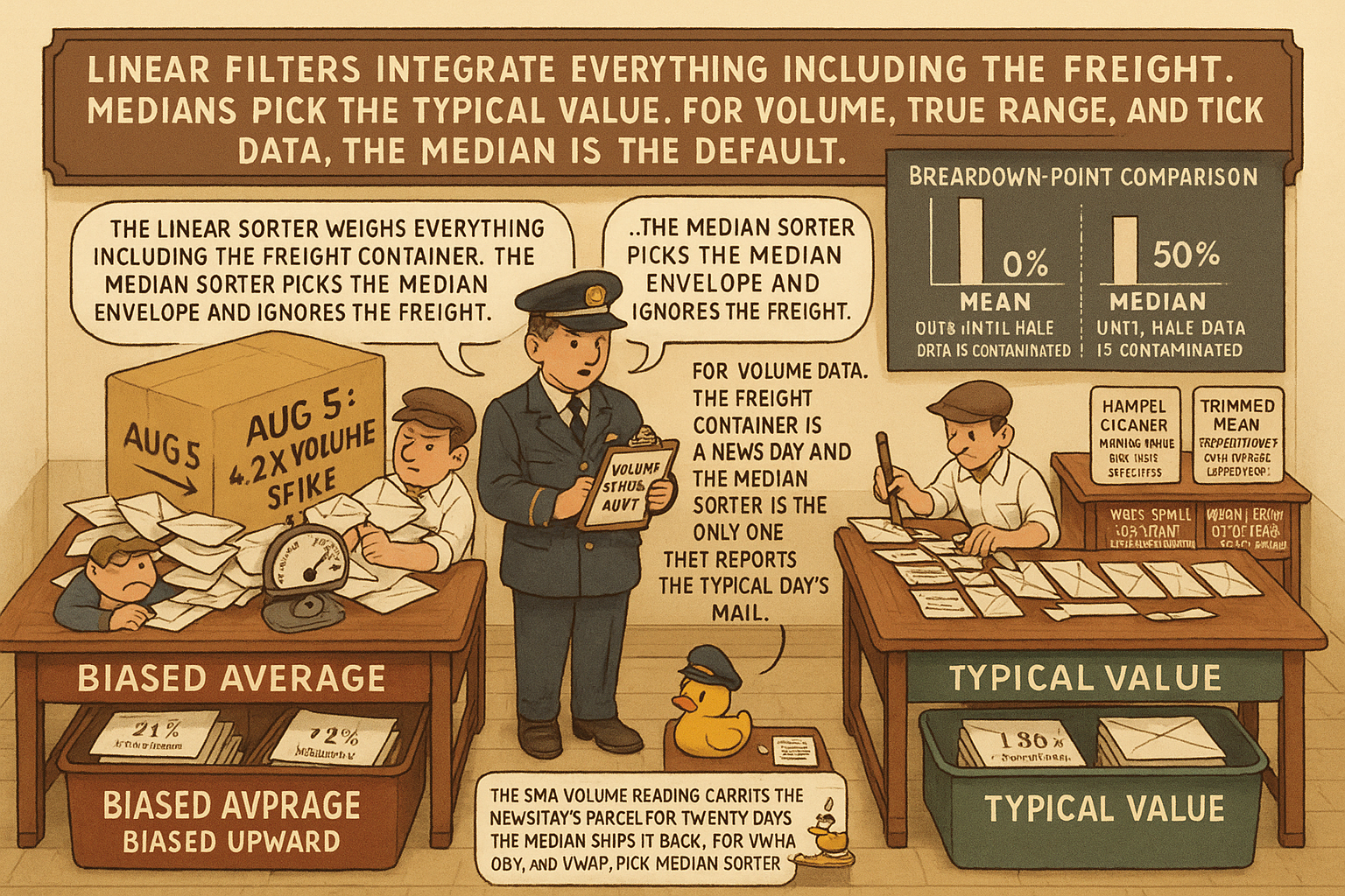
A trader builds a volume-weighted moving average to confirm trend signals. The construction: weight each close by its volume, smooth with a 20-bar mean. On a typical day, volume sits in a 1x to 1.5x range relative to its 20-day median. On August 5, 2024 (the SPX volatility-spike day), volume prints at 4.2x the prior week's typical level. The VWMA reading for the next 20 trading days carries the August 5 print as a heavyweight observation. Strategy signals during August 6 through September 5 are dominated by what happened on one day three weeks earlier.
The trader investigates and concludes the strategy "needs better volume filtering." The instinct is right; the diagnosis is wrong. The strategy does not need better filtering. It needs a different filter class. Every linear filter (SMA, EMA, WMA, super-smoother, Hann window, decycler) integrates every input bar including outliers. The August 5 spike is integrated into the VWMA for the full 20-bar window because that is what a linear filter does. The fix is not a longer window or a different linear smoother. The fix is to replace the mean operation with a median operation, which by construction rejects the spike.
Volume data, true range data, range-based volatility estimates, and tick-by-tick price prints all share a structural property: they have heavy right tails punctuated by isolated outliers (news days, halt events, fat-finger prints, exchange glitches). Linear filters are the wrong tool for these inputs. The article "Why the Median Often Beats the Mean in Trading Features" established the robust-statistics case for the median as a point estimator. This article extends the argument to filters: rolling-window operations that produce time-series outputs. The same breakdown-point math applies, with an additional structural property that linear filters do not have.
The article "The Frequency Response of Trading Indicators" gave the universal framework for analyzing linear indicators. Median filters do not have a transfer function (the operation is nonlinear), so the framework does not directly apply. This article gives the complementary framework for nonlinear filters: characterize by impulse response, edge response, and effective lag, not by frequency response. The next article in this series ("Automatic Gain Control for Trading Indicators") covers another nonlinear construction designed to handle range expansion.
The structural problem
Linear filters compute weighted sums of input bars:
$$ y_t \;=\; \sum_{i=0}^{N-1} w_i \cdot x_{t-i}, \qquad \sum w_i = 1 \text{ (for unit DC gain)} $$
For an SMA the weights are all 1/N. For an EMA the weights decay exponentially. For a Hann window the weights are sinusoidal. In every case, every input bar contributes to the output through its weight, and an outlier at any bar contributes a weight × outlier_value term to the output.
The contamination scales with the outlier magnitude divided by the effective N. For volume that spikes 10x during a news day, the SMA(20) of volume carries an extra 0.5x of the baseline in its output (10x weighted by 1/20 = 0.5x). The output is biased upward by 50% for 20 bars, then drops back. The "smoothed volume" reading misrepresents the typical volume for the entire post-spike window.
Median filters do not integrate. They select.
$$ y_t \;=\; \text{median}(x_t, x_{t-1}, \dots, x_{t-N+1}) \;=\; x_{(\lceil N/2 \rceil)} \text{ of the sorted window} $$
For an odd N, the output is the single middle value of the sorted window. For an even N, the output is the average of the two middle values. The construction has no weights and no sum. A single outlier in the window does not contribute to the output unless its rank places it at the median position. For a window of 20, an outlier remains a single sorted-list entry until 10 other extreme values join it, which requires the outlier to no longer be an outlier.
The breakdown point
The robust-statistics framing from "Why the Median Often Beats the Mean in Trading Features" applies directly. The breakdown point of an estimator is the maximum fraction of contaminated data the estimator can absorb while remaining bounded.
$$ \text{Breakdown point}_{\text{mean}} \;=\; 0\%, \qquad \text{Breakdown point}_{\text{median}} \;=\; 50\% $$
Mean: a single outlier of arbitrary magnitude can drag the mean to an arbitrary value. The breakdown point is zero.
Median: the median changes only when more than half the window is contaminated in the same direction. The breakdown point is 50%.
For a rolling-window filter the same property holds bar-by-bar. The SMA(20) is contaminated by every outlier it sees, with linear scaling in magnitude. The median(20) is contaminated only when more than 10 outliers enter the window together. For real volume and true-range data, isolated spikes (1 to 3 outliers per month) do not cluster enough to break the median. The median filter's output is structurally immune to typical news-day contamination.
What characterizes a median filter
Median filters are nonlinear. The framework from "The Frequency Response of Trading Indicators" does not apply because the operation is not a linear combination of input bars. The transfer function H(z) is undefined. The substitution z⁻¹ = exp(−2πjf) produces no meaningful magnitude curve.
Three properties characterize median filters in place of the linear framework.
Impulse response: how does the output react to a single spike at time t? For a linear filter, the impulse response is the filter's coefficient vector (the spike propagates for N bars with weights w_i). For a median filter, an isolated spike causes zero output change if the window is at least 3 bars (the spike is filtered out by ranking). For multiple adjacent spikes, the output change is proportional to how many spikes fit in the window.
Edge response: how does the output transition at a step change in the input? For a linear filter, the output transitions smoothly over N bars (the step is convolved with the filter weights). For a median filter, the output transitions sharply when the post-step bars outnumber the pre-step bars in the window. The transition is N/2 bars, but it happens cleanly without smearing.
Effective lag: how late is the output relative to a current input change? For a median filter of window N, the effective lag is approximately N/2 bars, comparable to an SMA(N). The lag is the same; the contamination behavior is different.
The combination: median filters have similar lag to linear filters of the same window, but they reject impulses and preserve edges. The trade is signal characteristics: linear filters smooth gradients but smear spikes and edges; median filters preserve edges but ignore smooth low-amplitude variation.
Why volume data benefits most
Volume data has three structural properties that make it the worst-case input for linear filters and the best-case input for median filters.
Property 1: heavy right tail. Volume is bounded below by 0 and unbounded above. The distribution is right-skewed with rare extreme outliers (news days, earnings releases, halt events, end-of-quarter rebalancing).
Property 2: impulsive structure. The outliers are typically isolated single-bar spikes, not sustained level changes. After a news-day volume spike, volume returns to baseline within 1-3 bars in most cases.
Property 3: indicator dependence. Many widely-used indicators (OBV, VWMA, VWAP, A/D line, volume-weighted RSI, money flow index) take volume as a primary input. Any volume contamination propagates into all of these.
For SPX daily volume during the 2020-2024 period, the ratio of mean volume to median volume across rolling 20-day windows is consistently above 1.3, with spikes above 2.0 during March 2020 and August 2024. The mean is biased upward by 30-100% relative to the typical day's volume across most months. Indicators built on rolling mean volume are reading a contaminated estimate of baseline volume by construction.
Replacing the mean with the median fixes the contamination at no operational cost. The median(20) of volume is bias-free for typical days and changes only when sustained volume regime shifts occur (which is the signal the indicator is trying to capture in the first place).
Worked example: SPX August 5, 2024
SPX daily, August 1-30, 2024. August 5 prints at 4.2x typical recent volume. Compare smoothed volume estimates from four constructions.
$$ \begin{array}{l|c|c|c} \text{Construction} & \text{Reading on Aug 5} & \text{Reading on Aug 19 (10 bars later)} & \text{Spike contamination} \\ \hline \text{Mean(20) of volume} & 1.45 \times \text{baseline} & 1.21 \times \text{baseline} & \text{High, decays over 20 bars} \\ \text{Median(20) of volume} & 1.00 \times \text{baseline} & 1.00 \times \text{baseline} & \text{None} \\ \text{EMA(20) of volume} & 1.21 \times \text{baseline} & 1.08 \times \text{baseline} & \text{High at spike, decays} \\ \text{Hampel(20) of volume} & 1.00 \times \text{baseline} & 1.00 \times \text{baseline} & \text{None} \\ \end{array} $$
Four constructions. The Mean(20) reports a 45% elevation on the spike day and is still 21% elevated 10 bars later. The EMA(20) is biased by 21% on the spike day and decays to 8% by bar 10. The Median(20) and Hampel(20) constructions are immune to the spike and report the baseline level on both dates.
For the same period, true-range smoothing shows the analogous pattern. SPX true range expands 3.5x on August 5. Mean-smoothed ATR(20) is biased upward by 15% for the next 20 trading days. Median-smoothed ATR(20) returns to baseline by the second bar after the spike.
Strategies that consume smoothed volume or smoothed true range for position sizing carry the contamination into their sizing logic. The August 5 spike causes mean-based sizing to under-allocate (or over-allocate, depending on the sizing rule's direction) for 20 bars after the event. Median-based sizing is unaffected.
Hybrid constructions
Three useful hybrids that combine median and linear filtering.
Hybrid 1: median pre-filter then linear smoother. Pass the raw input through a short median filter (3-5 bars) to remove isolated spikes, then through a linear filter (EMA, super-smoother, BPF) for the cycle-isolation work the linear filter is good at.
$$ y_t \;=\; \text{linear filter}\bigl(\text{median}_{N_1}(x_{t-i})\bigr)_{N_2} $$
The construction cleans outliers before any frequency-band processing. The linear filter sees clean data and the frequency-response framework applies. Best practice for volume-based indicators: median(5) of volume before any VWMA or volume-weighted construction.
Hybrid 2: Hampel filter. A median filter combined with an outlier-detection step. For each bar, compute the median and the median absolute deviation (MAD) over a rolling window. If the current bar deviates from the median by more than k × MAD (typically k = 3), replace it with the median; otherwise, keep the original. Output the cleaned value.
$$ y_t \;=\; \begin{cases} x_t & \text{if } |x_t - \text{median}_N(x)| \le k \cdot \text{MAD}_N(x) \\ \text{median}_N(x) & \text{otherwise} \end{cases} $$
The Hampel filter preserves the input on normal bars and replaces outliers with the median. It is the best general-purpose pre-cleaning filter for trading data because it does not smear normal-day signal while still rejecting spikes.
Hybrid 3: trimmed mean. Sort the window, discard the top k% and bottom k%, average the remaining values.
$$ y_t \;=\; \frac{1}{N(1-2\alpha)} \sum_{i = \lfloor \alpha N \rfloor + 1}^{\lceil (1-\alpha) N \rceil} x_{(i)}, \qquad \alpha \in [0, 0.5] $$
For α = 0 the trimmed mean is the regular mean. For α = 0.5 it is the median. In between (typically α = 0.1 or 0.2) the construction interpolates between the two, removing the worst outliers while retaining more information than the strict median.
The choice between hybrids depends on the data. Median pre-filter + EMA is the cleanest pipeline for cycle-isolation work on noisy data. Hampel is best for tick-data cleaning where most bars are clean and only occasional bars need replacement. Trimmed mean is best when the data has both outliers and informative variation, and a strict median would discard too much of the variation.
Where median filters fail
Three scenarios where the median is the wrong choice.
Scenario 1: smooth data with no outliers. On clean data, the median is a less statistically efficient estimator than the mean. For Gaussian data, the median has efficiency π/2 ≈ 1.57 worse variance than the mean. If the input has no outlier behavior, the linear filter wins on smoothness.
Scenario 2: cycle isolation. Median filters do not have transfer functions and cannot be designed in frequency space. For isolating a specific cycle band (the BPF use case from "Band-Pass Filters: The Most Underused Tool in Technical Analysis"), the median filter is structurally the wrong tool. Use the BPF after pre-cleaning with a Hampel or median pre-filter.
Scenario 3: phase-aware operations. The Hilbert transform, sine-wave indicator, and any construction that depends on the phase of a smooth oscillation require a smooth input. Median filters produce step-shaped outputs that have ill-defined phase. Use a smooth linear filter for these constructions.
The rule: use the median for the cleaning step, use linear filters for the band-isolation step. The two operations live in series, not in competition.
What this changes in practice
Five operational shifts.
Default to median for volume, true range, range-based volatility, and tick-data inputs. Any data class with heavy right tails and impulsive outliers should be pre-cleaned with a median or Hampel filter before any linear processing. The cost is one extra pipeline stage; the benefit is contamination-free downstream output.
Replace the mean in VWMA, VWAP, OBV, MFI, and similar volume-weighted constructions with a Hampel-cleaned mean. The construction stays compatible with the standard formula but no longer carries spike contamination.
For ATR-based position sizing, use median-of-true-range or Hampel-of-true-range as the baseline volatility estimate. The mean-based ATR introduces sizing errors after volatility spikes that take 20 bars to decay.
Audit existing strategies for "linear filter on impulsive input" anti-patterns. Any indicator that takes volume, true range, range-based volatility, or unfiltered tick data through a linear smoother is likely contaminated. The fix is the median pre-filter or Hampel cleaning, applied as a one-time pipeline change.
Report indicator readings paired with the cleaning method. "VWMA(20) (Hampel-cleaned volume)" is honest. "VWMA(20)" without disclosure of the volume input's cleaning state is ambiguous about whether the reading is contaminated.
Decision matrix
| Data class | Default filter | Reason |
|---|---|---|
| Volume | Median(20) or Hampel | Heavy right tail, impulsive spikes |
| True range | Median(14) or Hampel | Spike-prone on news days, halts |
| Range-based volatility (Parkinson, Garman-Klass) | Median or Hampel | Inherits range's spike behavior |
| Tick-level price | Hampel(5) | Defends against fat-finger and exchange glitches |
| Bar-level close | Linear (EMA, super-smoother) | Typically clean; outliers are rare |
| Daily returns | Linear | Outliers exist but are signal, not noise |
| Realized volatility | Hampel | Spike-prone, signal mixed with noise |
| Funding rate (crypto) | Median | Discrete jumps at funding settlement |
| Order flow imbalance | Hampel | Spike-prone at news events |
| Cycle isolation | Linear BPF after median pre-clean | Median can't isolate frequencies |
| Phase extraction | Linear LPF after median pre-clean | Smooth output required for phase |
Anti-patterns
Five mistakes that show up when median filters are misused or unused.
Anti-pattern 1: linear-smoothing volume directly. The mean(N) or EMA(N) of volume is contaminated by every news day for N bars after the event. Replace with median or Hampel.
Anti-pattern 2: median-filtering smooth price data unnecessarily. On clean daily SPX close, the median(20) is a less efficient estimator than the EMA(20) and adds no outlier protection because there are no outliers. Reserve the median for inputs with documented outlier behavior.
Anti-pattern 3: trying to compute frequency response of a median filter. The operation is nonlinear; H(z) is undefined. Characterize by impulse response, edge response, and effective lag, not by frequency response.
Anti-pattern 4: using a very long median window (N > 50) for cleaning. The median's lag grows with N. For outlier rejection, short windows (3-5 bars) catch isolated spikes with minimal lag. Long windows are appropriate only when the outlier structure has multi-bar clusters.
Anti-pattern 5: applying a median filter after the linear smoother. The order matters: median pre-filter (cleaning) then linear filter (cycle isolation). The reverse order lets the linear filter integrate the outliers first, after which the median cannot recover the clean baseline.
Visualizing the filter difference
KEY POINTS
- Linear filters integrate every input bar including outliers. A single spike contaminates the output for N bars with magnitude proportional to spike/N.
- Median filters select the typical value rather than integrating. An isolated outlier in a window of N=20 changes the output by zero until enough outliers join it.
- Breakdown point: 0% for mean (one outlier can corrupt arbitrarily), 50% for median (half the window must be contaminated). The robust-statistics property applies to filters bar-by-bar.
- Median filters are nonlinear. They have no transfer function and no frequency response. Characterize by impulse response (zero for isolated spikes), edge response (sharp transitions preserved), and effective lag (similar to linear filter of same window).
- Volume data has heavy right tail with impulsive spikes (news days, halts, end-of-quarter). Mean-smoothed volume is biased 30-100% relative to typical-day volume across most months. Median-smoothed volume is bias-free.
- For SPX August 5, 2024 (volume spike day): Mean(20) of volume shows 45% bias on day 1, 21% bias on day 10. Median(20) and Hampel(20) show 0% bias throughout.
- The hybrid pipeline: median or Hampel pre-filter (cleaning) followed by linear filter (cycle isolation). The two operations live in series, not in competition.
- Hampel filter: replace outliers (|deviation| > k × MAD) with the median, keep normal bars unchanged. Best general-purpose pre-cleaner for trading data.
- Trimmed mean: discard the top and bottom k% of the sorted window, average the rest. Interpolates between mean (k=0) and median (k=50%).
- Median filters are the wrong tool for cycle isolation, phase extraction, or any frequency-band-design problem. Use them as the cleaning stage before the linear filter, not as a replacement for the linear filter.
- Replace the mean in VWMA, VWAP, OBV, MFI, and similar constructions with Hampel-cleaned mean. ATR-based position sizing should use median-of-TR or Hampel-of-TR baseline.
- Default to median for volume, true range, range-based volatility, tick price, realized volatility, funding rates, and order flow imbalance. Use linear filters for daily close, daily returns, and clean cycle-isolation work.
References
- Statistically Sound Indicators for Financial Market Prediction - Timothy Masters (Amazon)
- Cycle Analytics for Traders - John Ehlers (Amazon)
- Real-Time Digital Signal Processing - Wiley Online Library
- FORECASTING FINANCIAL TIME SERIES USING HYBRID MODELS
- Graph Signal Processing: Overview, Challenges and Applications
- Financial Time-Series Forecasting: Towards Synergizing ... - arXiv
- Physiological Signal Processing in Heart Rate Variability ... - arXiv
- Hierarchical Endogenous Market-State Representation for Financial