2.26 The Frequency Response of Trading Indicators
Every linear indicator is a filter with a unique frequency response. RSI(14), MACD(12,26), Stochastic(14) read the same 15-40 bar cycle band three different ways. The confluence is redundancy.
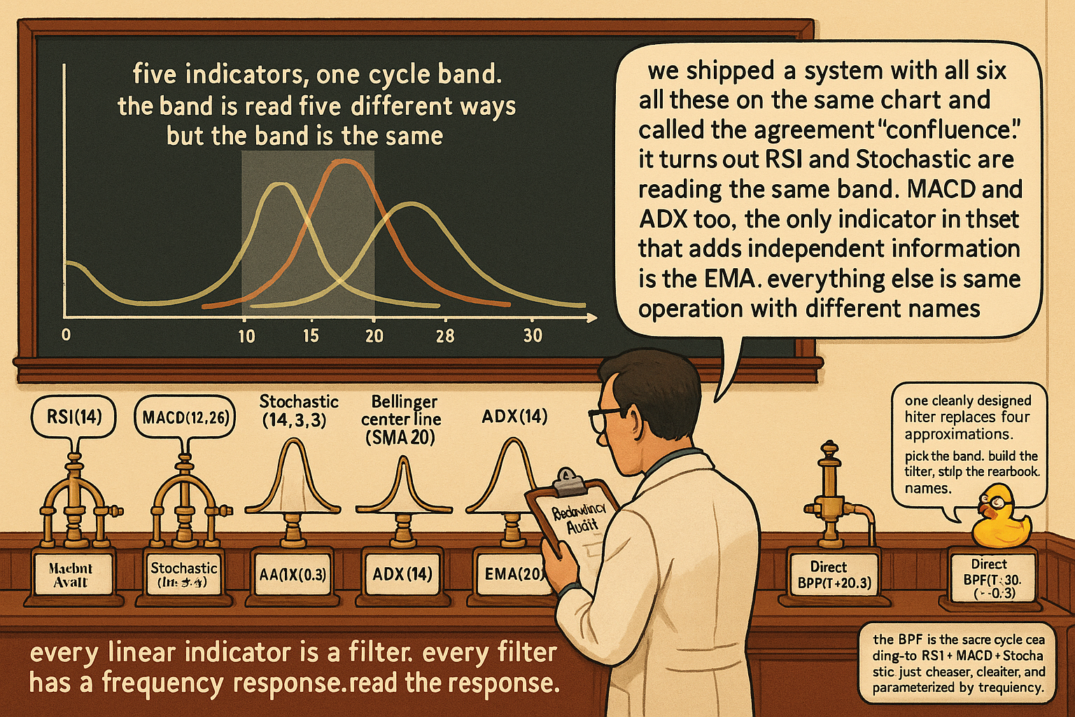
A trader stacks RSI(14), MACD(12, 26, 9), and Bollinger Bands(20, 2) on the same chart. The three indicators "look different," so the trader assumes they carry independent information and uses all three for confluence signals. The system trips because the indicators agree most of the time, disagree at the noisy edges, and the disagreement is treated as a high-conviction signal that turns out to be uncorrelated noise.
The structural problem: nobody computed what frequency content each indicator passes. RSI(14) and Stochastic(14) are nearly identical band-pass-ish operations on the same data. MACD(12, 26) and close-minus-EMA(20) target almost the same cycle band. Three "different" indicators are reading the same cycle component three different ways and calling the redundancy "confirmation."
Frequency response is the ground-truth description of every linear indicator. The magnitude of the transfer function evaluated on the unit circle (substitute z⁻¹ = exp(−2πjf) and take the modulus) gives a curve from frequency zero to the Nyquist frequency that tells you exactly which cycles the indicator passes, attenuates, or destroys. Two indicators with overlapping response curves carry duplicate information. Two indicators with disjoint curves carry independent information. The visual appearance on a chart is irrelevant to this question; the response curve is.
This article is the framework article for the filter-theory block. The prior articles in the series ("No Filter Is Predictive: What Traders Misunderstand About Smoothing", "Why the SMA Is Often a Terrible Smoother", "EMA vs SMA: Why Simplicity Still Matters", "The Trader's Guide to Low-Pass Filters", "High-Pass Filters for Traders", "Band-Pass Filters: The Most Underused Tool in Technical Analysis", "Decyclers: Extracting Trend by Removing Cycle Energy") each gave the response curve for a specific filter family. This article gives the universal recipe: how to compute the response of any linear indicator, what each region of the curve means, and how to use the framework to diagnose the standard TA toolkit. The next article ("How to Think About Indicator Lag Before Backtesting") turns the framework into a backtesting-cost discipline.
The recipe
Every linear indicator is a filter. Every filter has a transfer function expressed as a ratio of polynomials in z⁻¹:
$$ H(z) \;=\; \frac{b_0 + b_1 z^{-1} + b_2 z^{-2} + \dots + b_M z^{-M}}{a_0 + a_1 z^{-1} + a_2 z^{-2} + \dots + a_N z^{-N}} $$
The numerator coefficients (b_i) describe how the input contributes to the output. The denominator coefficients (a_j) describe how past output values contribute (the recursive part). For an FIR filter (no recursion), the denominator is just a_0. For an IIR filter (EMA, recursive HPF/LPF), both numerator and denominator are non-trivial.
To get the frequency response, substitute z⁻¹ = exp(−2πjf) where f is normalized frequency (cycles per bar, ranging from 0 at DC to 0.5 at Nyquist):
$$ H(f) \;=\; H(z)\,\Big|_{z^{-1} = e^{-2\pi j f}}, \qquad |H(f)| \;=\; \text{magnitude response} $$
The magnitude |H(f)| is the gain at each frequency. A magnitude of 1 means the cycle at frequency f passes through unchanged. A magnitude of 0 means the cycle is completely destroyed (a "zero" of the filter). A magnitude greater than 1 means the cycle is amplified. The full curve from f = 0 to f = 0.5 is the indicator's frequency response.
The reciprocal relationship between frequency and period gives the practical reading:
$$ T \;=\; \frac{1}{f}, \qquad f \;=\; \frac{1}{T} $$
A frequency of 0.05 corresponds to a 20-bar cycle. A frequency of 0.1 corresponds to a 10-bar cycle. A frequency of 0.5 corresponds to a 2-bar cycle (the fastest possible oscillation in discrete-time data, the Nyquist limit).
What each region of the curve means
Five structural readings.
DC gain (f = 0): the response to a constant (no-cycle) input. For a low-pass filter, DC gain is 1 (trend passes through). For a high-pass filter, DC gain is 0 (trend is cancelled). For a properly normalized band-pass filter, DC gain is 0 (trend cancelled, only the band passes).
Rolloff slope: how aggressively the filter attenuates frequencies outside the desired band. For a 1-pole LPF, the rolloff is 20 dB/decade above the cutoff. For a 2-pole LPF, it is 40 dB/decade. Steeper rolloff means better cycle isolation but more lag.
Zeros: frequencies where the response is exactly 0. The cycle at that frequency is completely destroyed. The SMA(N) has zeros at every multiple of 1/N (covered in the article "Why the SMA Is Often a Terrible Smoother"). The differencer (HPF with N=1) has a zero at DC. Zeros are structural and unavoidable for the filter that produces them.
Peaks: frequencies where the response is maximum. For an LPF, the peak is at DC. For an HPF, the peak is at Nyquist. For a BPF, the peak is at the center frequency. A peak above 1 means the filter amplifies the corresponding cycle, which is a design choice (resonant filters) or an artifact (sidelobes).
Sidelobes: secondary peaks outside the main passband. The SMA's sinc function has sidelobes that leak about 22% of nearby frequencies into the filter output. Hann and Blackman windows have much smaller sidelobes. The article "Why the SMA Is Often a Terrible Smoother" detailed the sidelobe critique.
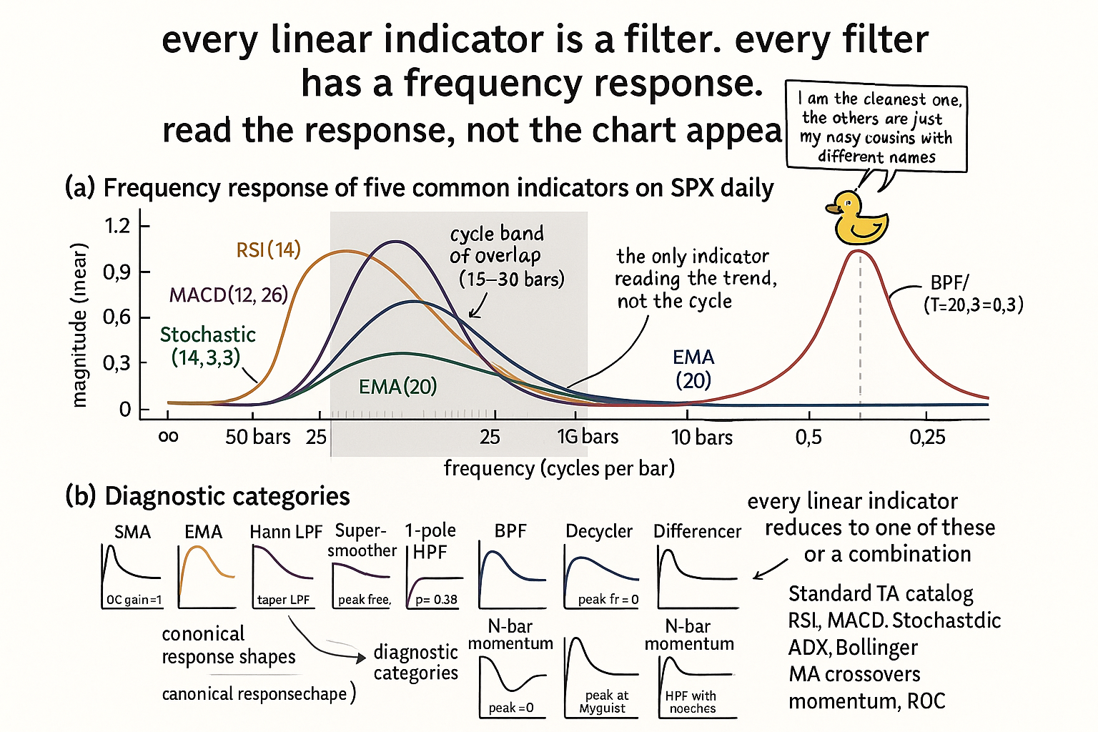
Catalog of canonical responses
The filter-theory block of this pillar produced a small set of distinct response shapes. Most of the TA indicator catalog falls into one of these shapes or a combination.
$$ \begin{array}{l|c|c|c} \text{Filter} & \text{DC gain} & \text{Nyquist gain} & \text{Shape} \\ \hline \text{SMA(N)} & 1 & 0 \text{ (if N even)} & \text{sinc with sidelobes, zeros at } 1/N, 2/N, \dots \\ \text{EMA(N)} & 1 & \approx \alpha/(2-\alpha) & \text{monotonic decay, no zeros, no sidelobes} \\ \text{Hann LPF(N)} & 1 & 0 & \text{tapered, sidelobes 32 dB down} \\ \text{Super-smoother(T)} & 1 & 0 & \text{2-pole LPF, critically damped, 40 dB/decade} \\ \text{1-pole HPF(T)} & 0 & 1 & \text{monotonic rise, complement of EMA} \\ \text{2-pole HPF(T)} & 0 & 1 & \text{steeper rise, 40 dB/decade} \\ \text{BPF(T, } \delta\text{)} & 0 & 0 & \text{peaked at frequency } 1/T \\ \text{Decycler(T)} & 1 & 0 & \text{equivalent to 1-pole LPF with HPF parameterization} \\ \text{Differencer (} x_t - x_{t-1}\text{)} & 0 & 2 & \text{HPF-like, amplifies highest frequencies} \\ \text{N-bar momentum (} x_t - x_{t-N}\text{)} & 0 & \le 2 & \text{HPF with notches at } k/N \\ \end{array} $$
Ten shapes. Every indicator in the standard TA literature reduces to one of these or to a combination produced by cascading (multiplying transfer functions) and parallel composition (adding transfer functions).
Diagnosing standard TA indicators
Apply the framework to the standard catalog. Each indicator's structural identity becomes clear once the underlying frequency response is computed.
RSI
The standard 14-period RSI is built from two operations: compute the bar-to-bar change (a 1-bar differencer, which is an HPF), separate gains and losses, then smooth each with an exponential average using α = 1/14. The final ratio is a non-linear transform of the smoothed gain and loss series, but the underlying linear structure is HPF cascaded with LPF.
The effective frequency response (treating the local linearization around moderate values) is a band-pass-like shape with peak around the 28-bar cycle and rolloff in both directions. The 1-bar differencer cancels DC; the EMA(14) smooths the very fast noise. The 14 in "RSI(14)" sets the EMA smoothing, not the differencer length.
The implication: RSI is approximately a band-pass filter on the cycle band centered around 28 bars. Two traders running "RSI(14)" and "BPF(T=28)" are reading the same cycle band through two different lenses.
MACD
MACD is the difference of two EMAs (EMA(12) minus EMA(26)). The transfer function is the algebraic difference:
$$ H_{\text{MACD}}(z) \;=\; H_{\text{EMA}(12)}(z) - H_{\text{EMA}(26)}(z) $$
At DC both EMAs have gain 1, so the MACD has DC gain 0 (trend is cancelled). At Nyquist both EMAs have gain ≈ α/(2−α), so the MACD has small Nyquist gain. The peak of the MACD response sits in the cycle band where the two EMAs disagree most, roughly at the 18-to-30-bar period.
The MACD is a band-pass filter built by EMA difference. The direct BPF construction does the same job with a single recursive section, lower lag, and explicit parameter control. The article "Band-Pass Filters: The Most Underused Tool in Technical Analysis" detailed the comparison.
Stochastic oscillator
Stochastic(N) computes (close − min_N) / (max_N − min_N) where min_N and max_N are the rolling minimum and maximum over N bars. The construction is nonlinear (the min and max are not linear operations), but the local linearization treats min_N + max_N as approximately a trend baseline. The Stochastic is then approximately close minus baseline, divided by range, which is a normalized HPF.
The Stochastic's effective frequency response is roughly an HPF with cutoff at frequency 1/N. The %K and %D smoothing (typically 3-period SMA on top) adds a mild LPF that turns the composite into a wide band-pass.
The implication: Stochastic(14, 3, 3) is approximately a band-pass on cycles around the 14-bar period, normalized to the [0, 1] range. RSI(14) and Stochastic(14) read nearly identical cycle bands and produce highly correlated outputs.
Bollinger Bands
The Bollinger Band center line is an SMA(20). The frequency response is the sinc function with zeros at every multiple of 1/20 = 0.05 (cycles of period 20, 10, 6.67, 5, ...). The 20-bar cycle is annihilated. The bands themselves are SMA ± k × rolling_std, which is nonlinear (rolling std is a quadratic operation).
The implication: Bollinger Bands inherit the SMA's sinc-and-sidelobe response in the center line. Any cycle near a 20-bar period or its harmonics is destroyed by the center line. The bands' width is a separate signal driven by the rolling std, which is not a linear filter response.
ADX
ADX is built on the True Range and Directional Movement components. True Range is a 1-bar nonlinear function of OHLC. Directional Movement is a 1-bar difference of high and low values. Both are then smoothed by an EMA with α = 1/14 for standard ADX.
The underlying linear structure is a 1-bar differencer cascaded with an EMA(14). The frequency response is similar to RSI: band-pass around the 28-bar period. ADX adds further nonlinear processing (max, abs, division) that shapes the output into a [0, 100] range but does not move the underlying cycle band.
The implication: ADX and RSI read approximately the same cycle band through different nonlinear lenses. The "directional" framing of ADX vs the "overbought-oversold" framing of RSI is interpretive, not structural; both indicators sit on the same cycle band.
Worked example: response curves overlaid
SPX daily. Plot the magnitude response of five indicators on a single chart, frequency axis from 0 to 0.25 (cycles per bar, equivalent to periods from infinity down to 4 bars).
$$ \begin{array}{l|c|c|c|c} \text{Indicator} & \text{Peak frequency} & \text{Peak period} & \text{DC gain} & \text{Band coverage} \\ \hline \text{RSI(14)} & 0.036 & 28\text{ bars} & 0 & \text{15-50 bars} \\ \text{MACD (12, 26)} & 0.042 & 24\text{ bars} & 0 & \text{16-40 bars} \\ \text{Stochastic(14, 3, 3)} & 0.05 & 20\text{ bars} & 0 & \text{12-30 bars} \\ \text{EMA(20) (as trend)} & 0 & \infty & 1 & \text{30+ bars} \\ \text{Super-smoother T=20 (as trend)} & 0 & \infty & 1 & \text{30+ bars} \\ \text{BPF(T=20, } \delta\text{=0.3)} & 0.05 & 20\text{ bars} & 0 & \text{17-23 bars} \\ \text{Close minus EMA(20)} & 0.05 & 20\text{ bars} & 0 & \text{8-30 bars} \\ \text{1-day momentum} & 0.5 & 2\text{ bars} & 0 & \text{2-6 bars} \\ \end{array} $$
Eight indicators. Five of them (RSI, MACD, Stochastic, BPF, close-minus-EMA) target overlapping cycle bands centered around 20-30 bar periods. Two (EMA, super-smoother) target the trend (DC and very low frequencies). One (1-day momentum) targets the fastest noise band.
The redundancy is now visible. RSI(14), MACD(12,26), and Stochastic(14) all sit in the 15-to-40-bar cycle band. A trader using all three is reading the same band through three nonlinear lenses. The "confluence" signal where all three agree is the signal that the 20-30-bar cycle is in a coherent phase; the disagreement signal is the noise from each indicator's nonlinear shaping.
The BPF(T=20, δ=0.3) is the narrowest and cleanest of the band-pass family. The close-minus-EMA(20) is the widest, with the most leakage. If the goal is to isolate the 20-bar cycle, the BPF is the structurally best choice. The RSI/MACD/Stochastic combo achieves no better band isolation than the single BPF and adds nonlinearity that obscures the underlying signal.
What this changes in practice
Five operational shifts.
Choose indicators by their frequency response, not by their lookback or their popular name. The frequency-response curve specifies what cycle bands the indicator reads. Two indicators with overlapping responses are redundant; two with disjoint responses are complementary.
Plot the response curve for every indicator entering the strategy. The plot is a 30-second computation (sample H(z) at 256 points along the unit circle, take the modulus). The plot reveals overlap, gaps, and miscalibration that no amount of chart inspection can show.
Compose indicators by composing transfer functions. Cascading two filters (output of one feeds the input of the next) multiplies their transfer functions. Parallel composition (sum or difference of two filter outputs) adds or subtracts their transfer functions. The compositions are designable in frequency space, not by trial and error.
Replace nonlinear-but-structurally-redundant indicators with their underlying linear equivalents. RSI(14), MACD(12,26), Stochastic(14) are all approximately the same band-pass operation. Pick one if cycle-band reading is the goal; pick the direct BPF if cleaner isolation matters.
Detect band gaps. If the indicator suite covers the 15-to-40-bar band heavily but ignores the 5-to-15-bar band entirely, the strategy is blind to faster cycles. The response-curve overlay reveals coverage gaps that ad-hoc indicator stacking cannot expose.
Decision matrix
| Goal | Recommended response shape | Recommended construction |
|---|---|---|
| Smooth trend, minimal lag | LPF with steep rolloff, DC gain 1 | Super-smoother or Hann window |
| Detrend, keep deviations | HPF, DC gain 0 | 1-pole HPF or 2-pole HPF |
| Isolate specific cycle band | BPF, peak at target frequency | Direct BPF |
| Cancel specific cycle | LPF with zero at target frequency | Decycler at cycle period |
| Trend-cycle decomposition | LPF + HPF pair, sum to 1 | Decycler + matched HPF |
| Multi-band cycle decomposition | Bank of BPFs at multiple T | Bank of direct BPFs |
| Predictor: not possible with linear filter | N/A | See "No Filter Is Predictive: What Traders Misunderstand About Smoothing" |
Anti-patterns
Five mistakes when working without the frequency-response framework.
Anti-pattern 1: stacking indicators with overlapping response bands and calling the agreement "confirmation." The agreement is structural redundancy. Reduce to one band-pass per cycle band of interest.
Anti-pattern 2: picking lookbacks by trial and error on backtest performance. The lookback maps to a cutoff frequency that should be chosen by what cycle band the strategy targets, not by what produces the highest historical Sharpe. The article "How to Think About Indicator Lag Before Backtesting" covers the discipline.
Anti-pattern 3: assuming an indicator's named "type" (RSI, Stochastic, MACD) maps to a unique frequency-response shape. RSI(14), Stochastic(14), and ADX(14) all sit in the same cycle band. The names are interpretive, not structural.
Anti-pattern 4: treating nonlinearity as if it produces a different cycle response. The nonlinear shaping in RSI (gain/loss separation) and Stochastic (range normalization) changes the output's distribution but does not move the underlying cycle band the indicator reads. The band is set by the linear components inside the construction.
Anti-pattern 5: building indicator "confluence" rules without computing the response overlap. Two indicators that always agree are one indicator with two names. Confluence rules built on this are over-counting evidence.
Visualizing the response
KEY POINTS
- Every linear indicator is a filter. Every filter has a transfer function H(z) and a magnitude response |H(f)| = |H(z)| evaluated on the unit circle.
- The magnitude response curve from f = 0 (DC) to f = 0.5 (Nyquist) is the ground-truth description of what cycle bands the indicator passes, attenuates, or destroys.
- Five regions to read on any response curve: DC gain (trend response), Nyquist gain (high-frequency response), zeros (cycles destroyed), peaks (cycles amplified or selected), rolloff slope (how aggressively cycles outside the band are rejected).
- The standard TA catalog reduces to a small number of canonical shapes: SMA (sinc with sidelobes), EMA (monotonic decay), Hann/Blackman LPFs (tapered), super-smoother (steep LPF), HPFs, BPF, decycler, differencer, N-bar momentum.
- RSI(14), MACD(12, 26), Stochastic(14, 3, 3), and ADX(14) all sit in approximately the same cycle band (15-40 bar periods). Stacking them is structural redundancy disguised as confluence.
- Bollinger Bands inherit the SMA's sinc-and-sidelobe response in the center line. The 20-bar cycle is annihilated by the SMA(20).
- MACD is algebraically a band-pass filter built by EMA difference. The direct BPF does the same job with lower lag and explicit parameter control.
- Choose indicators by their frequency response, not by their popular name or by a lookback chosen via backtest hyperparameter search.
- Compose indicators by composing transfer functions (multiplication for cascade, addition for parallel). Cascading two LPFs gives a 2-pole LPF; adding an HPF to a decycler reconstructs the original signal.
- Replace nonlinear-but-redundant indicators with their underlying linear equivalents. RSI/MACD/Stochastic are approximately the same band-pass operation; pick one or use the direct BPF.
- Plot the response curve for every indicator entering a strategy. The plot is a fast computation and reveals overlap, gaps, and miscalibration that chart inspection cannot show.
References
- Statistically Sound Indicators for Financial Market Prediction - Timothy Masters (Amazon)
- Cycle Analytics for Traders - John Ehlers (Amazon)
- Digital Signal Processing, System Analysis and Design, 2nd Edition
- FINANCIAL TIME-SERIES PREDICTION USING DEEP LEARNING
- 3 - Techniques for the synthesis of multi-band transfer functions
- Digital Signal Processing: System Analysis and Design
- FORECASTING FINANCIAL TIME SERIES USING HYBRID MODELS
- Filtering and Deconvolution (Chapter 13) - Quantitative Methods of
- Introduction to Real-Time Digital Signal Processing
- Continuous and Discrete-Time Filters: A Unified Operational ... - arXiv