3.2 Slow Wandering: The Most Dangerous Type of Market Change
Slow drift is harder to detect than abrupt breaks because standard tests have weak power against it. CUSUM and long-vs-short divergence catch what ADF misses. Trust the alarm when it triggers.
A trader builds a long-only momentum system on US large-cap equities. The signal is the 12-month total return minus the 1-month total return, ranked across the S&P 500 universe, top decile held equal-weight, rebalanced monthly. Backtest 1995 to 2010: Sharpe 0.71, annualized return 11.4%, max drawdown 32% (in 2009). Backtest 1995 to 2015 with the same rules: Sharpe 0.62. Backtest 1995 to 2020: Sharpe 0.48. Backtest 1995 to 2025: Sharpe 0.31. The strategy never had a single year of catastrophic failure. It had a slow, monotone deterioration of the edge. The trader who deployed it in 2010 captured most of the original edge. The trader who deployed it in 2018 captured a third of it. The trader who deployed it in 2024 captured roughly nothing.
Nothing broke. The trade-execution stack worked. The signal definition was unchanged. The universe was unchanged. The rebalance frequency was unchanged. The only thing that changed was the underlying joint distribution of (12-1 momentum, forward 1-month return) across the S&P universe. The slope of the conditional expectation flattened by approximately 0.04 standard deviations per year. Over fifteen years that is 0.6 standard deviations of edge silently erased.
This is slow wandering. The prior article in the publication ("Stationarity: The Word Every Trader Ignores Until It Kills the Strategy") covered the broad case for stationarity discipline and named slow drift as the failure mode that standard tests miss. This article gives slow wandering its own treatment because the diagnostic problem is different from the abrupt-regime problem and most testing machinery in the trader's toolkit is calibrated against the wrong threat. Abrupt breaks are noisy and obvious. Slow drift is silent and accumulates. The trader who only watches for abrupt breaks loses to slow drift on the strategies that survive long enough for the drift to matter.
What slow wandering is
Slow wandering is non-stationarity in which the parameters of the data-generating process drift slowly relative to the within-window noise. Formally, decompose the feature into a slowly-varying mean and a fast-varying residual.
$$ X_t = \mu(t) + \varepsilon_t, \qquad \mu(t) - \mu(t - W) = \delta \cdot W, \qquad \text{Var}[\varepsilon_t] = \sigma_W^2 $$
The drift rate δ is the change in the mean per unit time. The within-window noise σ_W is the standard deviation of the residual on the rolling window of length W. Slow wandering is the regime where δ is small relative to σ_W per W, but the cumulative drift δ · T over the deployment horizon T is comparable to σ_W or larger. The strategy backtest sees the small per-window drift and treats it as noise. The strategy live performance pays the cumulative drift as a slowly accumulating loss.
The signal-to-noise ratio that determines whether a stationarity test detects the drift on a window of length W is the drift over the window divided by the noise on the window.
$$ \text{SNR}(W) = \frac{\delta \cdot W}{\sigma_W / \sqrt{W}} = \frac{\delta \cdot W^{3/2}}{\sigma_W} $$
The 3/2 power on W is the operational fact that determines everything that follows. To detect slow drift you need either a slower drift to be larger relative to short-window noise (impossible to control), or you need to use a longer window. Doubling the window length increases the SNR by a factor of approximately 2.83. Quadrupling it increases the SNR by a factor of 8. Standard ADF and KPSS implementations on 252-day or 1000-day windows have low power against drifts that take 5 to 10 years to fully express.
Why standard tests miss it
Three structural reasons.
Reason 1: window length. ADF, KPSS, and the rolling-mean check from the prior article are all run on a fixed window. The window is short enough to keep the test responsive to abrupt changes (typically 252 days, sometimes 1000) and long enough to give the test reasonable statistical power against fast drift. Slow drifts whose half-life is several years are below the detection floor of these tests at standard windows. Running the same tests on 5-year or 10-year windows raises detection power but trades responsiveness for it.
Reason 2: in-sample fitting absorbs the drift. When a strategy is fit (parameters tuned, thresholds calibrated) on a long historical window that contains the drift, the optimizer treats the drift as part of the noise structure. The fitted parameters are a compromise across the drift trajectory. The compromise looks reasonable on the in-sample data because the optimizer minimized over it, but the out-of-sample data is one more step along the drift path, not a fresh draw from the same distribution. The strategy underperforms its in-sample backtest by an amount proportional to the cumulative drift across the OOS window.
Reason 3: standard rolling-mean checks compare the rolling mean to itself, not to a long-run reference. A 252-day rolling mean of a slowly drifting feature traces the drift trajectory smoothly. The rolling mean does not look unusual at any single point. The drift only becomes visible when the rolling mean is compared to a much longer reference (a 5-year or 10-year mean, or a fixed pre-deployment baseline). The diagnostic that catches slow drift is not "is the rolling mean changing" but "is the rolling mean different from the mean of the regime we deployed against".
Where slow wandering shows up in markets
Four examples where the slow drift was the actual story and most operators noticed only after the strategy was already underperforming.
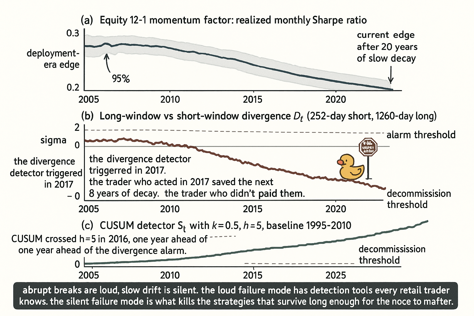
Example 1: equity momentum decay. The 12-1 momentum factor on US large-caps had a Sharpe of approximately 0.7 from the 1980s through the early 2000s, decayed to approximately 0.4 by the mid-2010s, and runs near 0.2 in the most recent decade. The factor was not killed by a single event. It was eroded by widening participation (more crowded trade), declining transaction costs (faster arbitrage), and a structural shift in the equity universe toward larger and lower-vol mega-caps that exhibit weaker momentum. None of these is a regime break in the abrupt sense. Each is a slow trend that compounded over decades.
Example 2: equity-bond correlation drift. Rolling 250-day correlation of SPX daily returns to 10-year Treasury daily returns ran negative through most of 2000 to 2020 (mean approximately -0.35), shifted to slightly positive around 2022 (mean approximately +0.10), and has stabilized around -0.15 in 2024 to 2025. The 60/40 portfolio's diversification benefit is a function of this correlation. The 2022 shift was partially abrupt and partially the culmination of slow drift in the macro regime (inflation expectations rising structurally). Strategies that assumed a stationary -0.35 correlation experienced surprising drawdowns proportional to the cumulative correlation drift.
Example 3: FX carry-trade decay. The G10 carry trade (long highest-yielders, short lowest-yielders) earned a robust premium through the 1980s and 1990s, decayed through the 2000s, and has produced near-zero risk-adjusted returns post-2008. The 2008 crisis is the convenient narrative, but the underlying driver was the slow convergence of central-bank policy rates across the developed world (the cross-sectional yield dispersion shrank from over 800 basis points in the 1990s to under 200 basis points by the late 2010s). The carry premium scales with the dispersion. A strategy that assumed historical carry returns were the relevant prior was making a stationarity assumption against a slow drift in the macro substrate.
Example 4: realized volatility long-run drift. SPX realized volatility on the 252-day rolling window has averaged approximately 16% across the post-1990 sample, but the conditional mean depends on the macro regime. The 1990s averaged around 14%, the 2000 to 2008 window averaged around 18%, the 2010 to 2019 window averaged around 14%, and the post-2020 window has averaged around 18%. Volatility-targeting strategies that normalize against a long historical mean carry the drift in their position-sizing rule. Strategies that use rolling estimates with too-short a window adapt fast but pay an estimation-noise tax. The trade-off between drift adaptation and estimation noise is operational and non-trivial.
Detecting slow wandering
Three detection tools. Each addresses a different failure mode of the standard tests.
Tool 1: long-window mean vs short-window mean divergence. Compute the rolling mean on two windows: a short window (252 bars) and a long window (1260 bars, approximately 5 years). Compute the divergence as the short-minus-long.
$$ D_t = \hat{\mu}_t^{(\text{short})} - \hat{\mu}_t^{(\text{long})}, \qquad D_t \text{ should be near zero under stationarity} $$
Under stationarity, D_t is mean-zero with a known standard deviation that depends on the window lengths. Under slow drift, D_t accumulates a non-zero expected value proportional to the drift rate. A persistent divergence of D_t in one direction across multiple short windows is the signature of slow drift. Standardize D_t by its theoretical stationary standard deviation and trigger an alarm when the standardized value exceeds 2 or 3 sigma persistently.
Tool 2: CUSUM chart. The cumulative sum of standardized deviations from a reference mean detects slow drift faster than the rolling-mean check.
$$ S_t = \max\!\left(0,\; S_{t-1} + \frac{X_t - \mu_0}{\sigma_0} - k\right), \qquad \text{alarm when } S_t > h $$
The reference mean μ_0 and reference std σ_0 are estimated from a clean baseline period (the strategy development window). The slack parameter k controls sensitivity to small drifts (typical k = 0.5 detects drifts of size 1·σ_0 efficiently). The threshold h controls the false-alarm rate (h = 4 to 5 is conservative). CUSUM was designed for industrial process control where slow drift is the dominant failure mode, and it transfers directly to the trading-feature monitoring problem. The detection delay for a drift of size d is approximately h / d in standardized units, which is order-of-magnitude faster than waiting for the rolling mean to visibly move.
Tool 3: Bayesian online change-point detection. A formal model of the drift hypothesis. Maintain a posterior distribution over the time of the last regime change. The posterior is updated with each new observation. When the posterior mass concentrates on a recent date, the algorithm has detected a change. This is more sensitive than CUSUM but requires more modeling commitment (priors on regime length, parametric form of the change). Useful when you need a probabilistic alarm rather than a binary one and have a clear prior on regime length.
The article "Volatility Regimes and Strategy Survival" later in this pillar covers the application of these tools to volatility specifically. The mechanics generalize to any feature whose mean or variance is at risk of slow drift.
Defending against slow wandering
Five operational defenses. Each addresses a different aspect of the problem.
Defense 1: continuous walk-forward. The article "Why Walk-Forward Testing Is Better Than One Big OOS Split" later in this pillar argues this in detail. The mechanism: retrain the strategy at quarterly or annual cadence so the in-sample window slides forward and absorbs the drift. The retrain is not a backtest; it is a recalibration of parameters against the most recent regime. The cost is parameter instability, which itself can be a sign of overfitting. Monitor the parameter trajectory and reject retrains that produce wild swings.
Defense 2: parameter aging. Apply an explicit half-life to the weight given to old observations. A strategy that uses an EWMA estimator with half-life of 2 years gives 50% weight to data more than 2 years old, 25% to data more than 4 years old, and so on. The half-life is a hyperparameter that itself overfits if chosen by backtest, but a fixed economically-motivated half-life (e.g., one business cycle) is a defensible prior. Parameter aging is the time-domain analog of rolling normalization (covered in "Rolling Normalization: Useful Tool or Hidden Overfit?").
Defense 3: multi-timescale regime detection. Run regime detection (CUSUM, Bayesian change-point, regime-switching model) at multiple timescales simultaneously. Short timescales (weeks to months) catch abrupt breaks. Long timescales (years) catch slow drift. The strategy gating layer combines both: disable on abrupt break, taper on slow drift. The tapering rule is operationally important: cut position size as the drift signal accumulates, rather than waiting for a binary disable trigger that may arrive years too late.
Defense 4: explicit decommission criteria. Every strategy has a written specification of the conditions under which it is shut down. The criteria include: cumulative drift on key features exceeds X sigma against the deployment baseline, OOS Sharpe falls below Y for Z consecutive months, drawdown exceeds the historical maximum by W%. The decommission decision is automatic against the criteria, not discretionary. The article "How to Detect When a Trading System Is Dying" later in this pillar gives the operational checklist.
Defense 5: portfolio-level finite-life budgeting. Assume each strategy has a finite life. Size each strategy's allocation so the portfolio survives the loss of any single strategy without catastrophic drawdown. Maintain a research pipeline of new strategies to replace dying ones. The article "Why Systems Work Until They Don't" frames this as the steady-state portfolio management problem rather than the one-time strategy-selection problem.
The trade-off: detection lag vs false alarms
Slow drift detection is a hypothesis-testing problem. Type I error is a false alarm (declaring drift when none exists, leading to unnecessary strategy decommissioning or retraining). Type II error is a missed detection (failing to declare drift, leading to silent edge erosion). The two errors trade off against each other through the detection threshold.
$$ \Pr(\text{false alarm} \mid \text{stationary}) = \alpha, \qquad \Pr(\text{detect} \mid \text{drift rate } \delta) = 1 - \beta(\delta) $$
For a CUSUM detector with threshold h, lowering h reduces detection lag (catch drift sooner) but raises false-alarm rate (more unnecessary decommissions). Raising h reduces false alarms but increases the time to detection (more cumulative loss before action). The right operating point depends on the cost ratio: how much edge do you lose per unit of detection delay versus how much do you lose by retraining or decommissioning a still-good strategy.
For most retail and small-shop quant operations, the cost of unnecessary decommission is high (rebuilding edge is expensive) and the cost of detection delay is moderate (the drift accumulates slowly by definition). This argues for conservative thresholds (h = 5 to 6, k = 0.5) and pairing CUSUM with multiple corroborating signals before taking action. For institutional operations with diversified strategy pools, the cost of unnecessary decommission is lower (other strategies are running) and the cost of detection delay is higher (concentrated risk). This argues for tighter thresholds and faster action.
Decision matrix
| Drift type | Detection tool | Defense | Speed of response |
|---|---|---|---|
| Abrupt regime break (1-day shock) | Z-score on daily change | Disable strategy on alarm | Same-day |
| Fast drift (weeks to months) | Rolling-mean check at 252-day window | Walk-forward retrain | Quarterly |
| Slow drift (1 to 5 years) | CUSUM with k=0.5, h=5 | Parameter aging + position taper | Annual |
| Multi-decade structural shift | Long-window vs short-window divergence | Decommission strategy | Multi-year |
| Mean drift | CUSUM on standardized feature | Rolling normalization | Per detector |
| Variance drift | CUSUM on log realized vol | ATR scaling on inputs | Per detector |
| Correlation drift | Rolling correlation vs long-run | Disable correlation-dependent rules | Quarterly |
| Distributional drift (shape change) | KS test on rolling distribution | Re-fit rank or sigmoid transforms | Annual |
The matrix is operational, not exhaustive. Each row pairs a class of non-stationarity with a detector and a defense. The detector and defense are matched to the speed of the drift, which is the parameter that determines what tools have power.
Anti-patterns
Five common mistakes specific to slow drift.
Anti-pattern 1: "ADF rejected, the feature is stationary." ADF on a 1000-day window has low power against drifts whose half-life exceeds 3 years. The test passes even when the cumulative drift across the deployment horizon will erase the strategy edge. Run the long-window vs short-window divergence and CUSUM to cover the slow-drift case explicitly.
Anti-pattern 2: "I'll backtest on a longer history to capture more regimes." A longer history captures more abrupt regimes, which is good. It also bakes in more cumulative drift, which is bad: the optimizer averages across a moving target and produces parameters that are a compromise across all the historical regimes, rather than tuned to the current regime. The right framing is to backtest on a long history for diagnostic purposes (does the strategy survive every individual regime?) and to fit parameters to a recent window (is the strategy tuned to the current regime?). The two questions need different windows.
Anti-pattern 3: "I'll use a 60-day rolling normalization to handle the drift." Sixty days is long enough to capture abrupt vol regime changes and short enough to track slow drift, which sounds ideal. The problem: a 60-day rolling normalization on a feature that has a multi-year cycle will track the cycle and remove the very signal that the strategy was supposed to trade. The cure becomes the disease. Match the rolling-window length to the drift timescale, not to the abrupt-shock timescale.
Anti-pattern 4: "The strategy underperformed for one year, but it always recovers." A single underperforming year on a slow-drift-decayed strategy looks identical to a normal drawdown on a still-healthy strategy. The discrimination requires the drift detection. Without the detection, the trader will hold a dying strategy through several underperforming years before noticing, and the held losses will be large. Run the detector. Trust the detector when it triggers. The detection logic, not the P&L, is the disable trigger.
Anti-pattern 5: "Strategy decay is the cost of doing business." It is the cost, but it is not an excuse to avoid measuring it. The trader who measures decay can decommission early and reallocate capital to fresh strategies. The trader who treats decay as an unmeasurable fact-of-life loses to the trader who measures it. The article "How to Detect When a Trading System Is Dying" frames the operational version of this discipline.
Visualizing slow wandering
KEY POINTS
- Slow wandering is non-stationarity in which the parameters of the data-generating process drift slowly relative to within-window noise. The cumulative drift across the deployment horizon is the loss; the per-window drift looks like noise.
- Detection power scales with W^(3/2) where W is the test window. Standard 252-day or 1000-day rolling tests have low power against drifts whose half-life exceeds 3 years.
- Three structural reasons standard tests miss slow drift: window length too short, in-sample fitting absorbs the drift into the parameter set, rolling-mean checks compare the rolling mean to itself rather than to a deployment-era baseline.
- Four real market examples: equity 12-1 momentum factor decay over 30 years, equity-bond correlation drift across 2020 to 2024, FX carry-trade decay across 1990 to 2010, SPX realized vol regime drift across decades. None had an abrupt break large enough for standard tests to catch as a single event.
- Three detection tools: long-window vs short-window divergence (cheap, intuitive), CUSUM (sensitive, designed for slow drift, fast detection), Bayesian online change-point (most sensitive, most modeling commitment).
- Five defenses: continuous walk-forward retraining, explicit parameter aging via EWMA half-life, multi-timescale regime detection running short and long detectors in parallel, written decommission criteria, portfolio-level finite-life budgeting that assumes every strategy dies eventually.
- The detection-lag vs false-alarm trade-off is set by the threshold h on the CUSUM (or analogous parameter on other detectors). Conservative thresholds favor avoiding unnecessary decommission. Tight thresholds favor catching drift early. The right operating point depends on the cost ratio of edge erosion vs decommission cost.
- Anti-pattern: ADF rejection treated as proof of stationarity. ADF rules out a unit root on the test window and is silent on slow drift below the test's power threshold.
- Anti-pattern: longer backtest window assumed to be safer. A longer window dilutes parameter fits across a moving target. Diagnostic backtest on long history, parameter fit on recent regime; two questions, two windows.
- Anti-pattern: a single underperforming year treated as a routine drawdown. A drawdown on a slow-decayed strategy looks identical to a normal drawdown. Run the drift detector and let the detector, not the P&L, drive the disable decision.
- The current article gives slow drift its own treatment because the detection problem is structurally different from abrupt-break detection. The next article in the publication ("Why Systems Work Until They Don't") generalizes the slow-drift framework to the steady-state question of strategy lifecycle: how to operate a portfolio of strategies that all eventually decay, and how to budget capital and research bandwidth around that finite-life assumption.
References
- Testing and Tuning Market Trading Systems - Timothy Masters (Amazon)
- Data Mining Algorithms in C++ - Timothy Masters (Amazon)
- Developing & Backtesting Systematic Trading Strategies
- Online Quantitative Trading Strategies - NYU Stern
- OptionMC: A Python package for Monte Carlo pricing
- How to Validate Trading Strategies Using Data - LuxAlgo
- Robustness Testing of Country and Asset ETF Momentum Strategies
- The GT-Score: A Robust Objective Function for Reducing Overfitting
- An Engineer's Guide to Building and Validating Quantitative Trading
- LLM-DRIVEN AUTOMATED ROBUST FEATURE ENGINEERING
- SysTradeBench: An Iterative Build–Test–Patch Benchmark for Drift‑Aware Systematic Trading
- Momentum Strategies: From Novel Estimation Techniques to Trading and Risk Management Applications
- Slow Momentum with Fast Reversion: A Trading Strategy Using Online Changepoint Detection
- Constructing Time-Series Momentum Portfolios with Deep Multi-Task Learning
- Combining Mean Reversion and Momentum Trading Strategies in Foreign Exchange Markets
- Modern Machine Learning Tools in Finance: A Critical Perspective
- Enhancing Time Series Momentum Strategies Using Deep Neural Networks
- The Intrinsic Instability of Financial Markets - arXiv