4. Market Structure Notes June 1, 2026 9 min

4.1 Noise Is Not Volatility

Two markets can show identical volatility and opposite tradeability. Volatility measures how far price moves; noise measures how much cancels out. Trade the noise axis, not the variance.

Take two markets over the same quarter. Market A is EURUSD: it closes the quarter 1.2% above where it opened, but the daily candles wander up and down so much that the price travelled a total absolute distance of roughly 18% to get there. Market B is a trending crude-oil run: it closes the quarter 14% higher and travelled a total absolute distance of 22% along the way. Measure each one with a standard 20-day annualized standard deviation and you get similar numbers, around 14% to 16% annualized. The volatility readings say these two markets are siblings. They are not. One delivered almost no net direction per unit of path travelled, and the other delivered direction efficiently. A trend system tuned to one will bleed on the other, and the volatility number told you nothing about which is which.

This is the distinction the rest of Pillar 4 is built on. Volatility measures how far price moves. Noise measures how much of that movement cancels itself out before producing any net direction. They are different quantities, they are driven by different mechanisms, and conflating them is the single most common reason a strategy that backtests well on one instrument dies on another that looks statistically identical. The article "Market Personality: Why Gold, FX, Crypto, and Equities Need Different Systems" used the efficiency ratio to fingerprint markets; this article isolates the underlying property that the efficiency ratio is measuring, and explains why you cannot read it off a volatility chart.

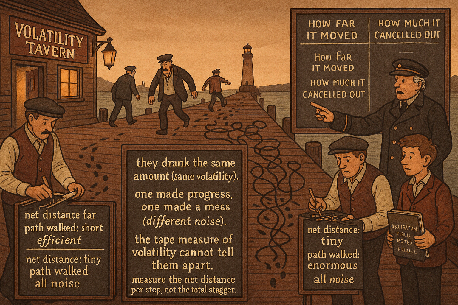
A drunk walking home covers a lot of ground. He staggers left, staggers right, lurches forward, drifts back. Measure his total foot-distance over an hour and it is large. Measure how far he ended up from where he started and it is small. A sober person walking the same hour covers less total foot-distance but ends up much further from the start. The drunk is high-noise, high-path, low-net. The sober walker is low-noise, lower-path, high-net. Volatility is the foot-distance. Noise is the staggering. Net direction is what you can actually trade.

Two markets, identical volatility, opposite personality

Here is the worked version, because the abstract claim does not land without numbers.

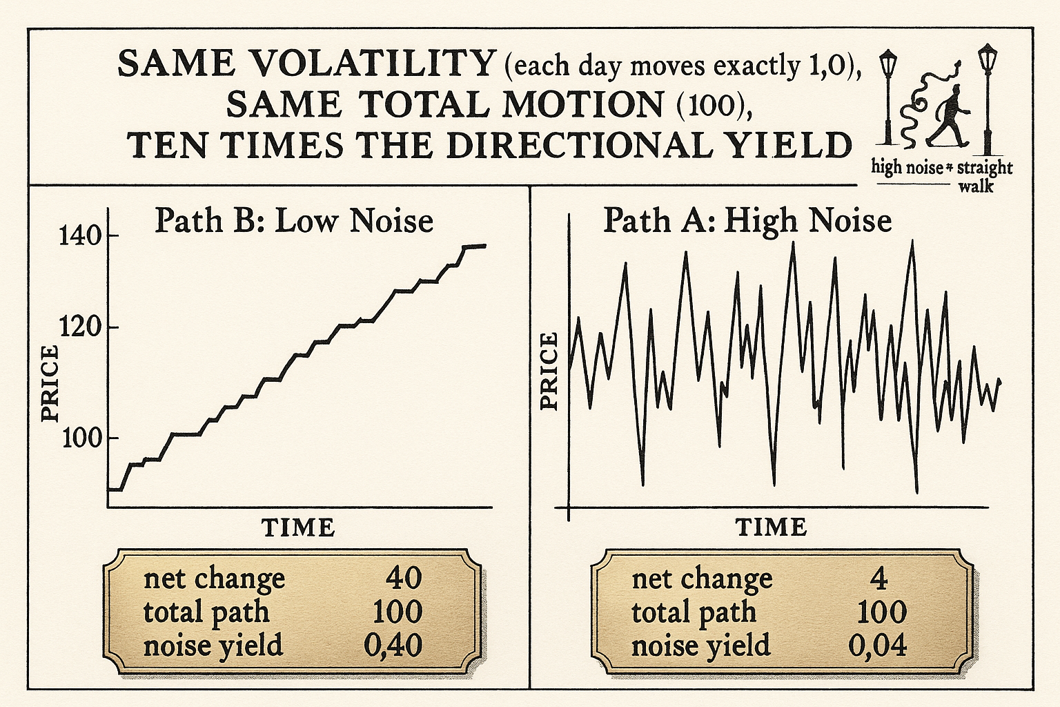
Construct two synthetic 100-day price paths, both starting at 100, both with daily moves of fixed magnitude 1.0 (so the day-to-day "volatility" is identical by construction; every single day moves exactly 1 point). Path A alternates direction with high probability: up, down, up, down, with occasional runs. Over 100 days it ends at 104. Path B keeps direction with high probability: long runs of up days broken by short pullbacks. Over 100 days it ends at 140.

Both paths have the same per-day absolute move (1.0), so the same realized volatility. The total path length is the same too: 100 days times 1.0 equals 100 points of absolute travel for each. The difference is entirely in how that 100 points of travel converted to net change. Path A converted 4 points net. Path B converted 40 points net. Same volatility, same total motion, a tenfold difference in directional yield.

The ratio of net change to total path length captures exactly this. For path A it is 4 divided by 100, equal to 0.04. For path B it is 40 divided by 100, equal to 0.40.

$$ \text{Noise-adjusted yield} = \frac{|P_{\text{end}} - P_{\text{start}}|}{\sum_{i=1}^{N} |P_i - P_{i-1}|} $$

The numerator is net directional change (where price ended versus where it started). The denominator is the sum of every individual day's absolute move, the total distance the price actually walked. A value near 1 means almost every step went in the same direction (a straight line, low noise). A value near 0 means the steps cancelled out (a drunk's walk, high noise). Volatility lives in the denominator alone; it has no idea what the numerator is doing. That is why two markets with the same denominator can have wildly different numerators, and why you cannot back out noise from a volatility reading.

Why the distinction is not academic

Three operational consequences follow directly, and each one costs money if ignored.

Consequence 1: trend systems harvest the numerator, not the denominator. A breakout or moving-average system profits when net directional change is large relative to the chop it has to sit through. Feed it a high-volatility, high-noise market (large denominator, small numerator) and it generates frequent signals that whipsaw, because the volatility triggers entries while the noise reverses them before they pay. The article "Why ATR Normalization Is More Than a Volatility Trick" handled the scaling problem; the noise problem is upstream of scaling and cannot be normalized away.

Consequence 2: mean-reversion systems harvest the denominator against the numerator. A fade or grid system profits when price oscillates a lot (large denominator) without committing to a direction (small numerator). High noise is the fuel. Feed a mean-reversion system a low-noise trending market and it sells every rip and buys every dip into a one-way move, accumulating a portfolio of losers that never revert. The article "Why Grid Systems Need Noise, Not Just Volatility" develops this; the precondition is the noise measurement, not the volatility measurement.

Consequence 3: volatility-targeting position sizing does not adjust for noise. If you size positions to a constant volatility target, you treat path A and path B as equally risky and equally tradeable. They are equally risky in the variance sense and completely different in the edge sense. Volatility targeting will hand the same capital to a market where your trend edge is zero as to one where it is strong, and the blended result will disappoint for reasons the risk report cannot explain.

What drives noise, and why it is more stable than volatility

Volatility is famously non-stationary; the article "Why Volatility Is More Non-Stationary Than Trend" documented how it clusters, spikes, and mean-reverts on its own clock. Noise behaves differently. The amount of directional persistence a market exhibits is tied to its participant structure and its information flow, and those change on a slower clock than volatility does.

Trade-flow structure sets the floor on noise. A market dominated by two-sided market-making and short-horizon liquidity provision (G10 FX intraday, large-cap equities at the tightest spreads) mechanically generates mean-reverting micro-structure: every aggressive buy is met by an inventory-adjusting sell, and the price oscillates around a slowly moving fair value. That produces high noise at short horizons regardless of how volatile the day is. A market dominated by slow directional flow (a commodity in a supply shock, a currency under a sustained central-bank divergence) generates persistence: the same direction repeats because the underlying imbalance repeats. That produces low noise even on quiet days.

Information arrival sets the spikes. News does not change a market's noise character; it changes its volatility. A surprise print can double the daily range without changing whether the subsequent moves persist or cancel. This is why you can have a high-volatility day inside a high-noise regime (a violent chop) and a low-volatility day inside a low-noise regime (a quiet grind higher). The two axes are close to independent.

The practical upshot: you can characterize a market's noise level over a few years and trust it to drift slowly, the way the article "Slow Wandering: The Most Dangerous Type of Market Change" framed slow regime drift. You cannot do the same with volatility, which can regime-shift in a week. Noise is a structural property; volatility is a state variable.

Measuring noise three ways

The yield ratio above is the most common noise measure, but it is one of three, and they agree often enough to cross-check each other.

Measure 1: the efficiency-style ratio (net change over total path length). Bounded between 0 and 1, cheap to compute, sensitive to the lookback window. This is the workhorse, developed in full in the next article, "Efficiency Ratio Explained for Traders".

Measure 2: price density (how much of the high-low box the price actually fills). A choppy market paints the whole box; a trending market leaves most of it empty. Covered in "Price Density: A Visual Way to Measure Market Choppiness".

Measure 3: fractal dimension (how space-filling the path is). A straight line has dimension near 1; a path that fills a plane approaches dimension 2. High noise pushes the dimension toward 2. It is the most expensive to estimate and the least stable on short windows, so it is a confirmation tool rather than a primary signal.

All three answer the same question: per unit of motion, how much net direction did I get? They differ in computation, not in intent. The discipline is to pick one as primary (the efficiency ratio) and use a second as a sanity check, because any single window-dependent estimate can mislead on a short sample, exactly the small-sample fragility the article "Trade-Count Thresholds for Backtest Reliability" warned about for performance metrics.

The classification mistake this prevents

The mistake is to read a volatility chart, see two markets at 15% annualized, and conclude they are interchangeable backtesting venues. That conclusion drives the "run it on everything" workflow the article "Why Works on All Markets Is Usually a Red Flag" criticized. The fix is to add the noise axis before deciding anything. A two-axis grid, volatility on one axis and noise on the other, separates four quadrants that demand different treatment.

	Low noise (efficient)	High noise (choppy)
Low volatility	Quiet grind: trend systems, small size	Quiet chop: mean-reversion, scalping
High volatility	Violent trend: trend systems, vol-scaled size	Violent chop: fade with caution, wide stops

The two columns are the strategic divide; the two rows are the sizing divide. Volatility tells you how big to bet. Noise tells you what game you are playing. Get the column wrong and no amount of getting the row right will save the strategy.

Visualizing noise versus volatility

KEY POINTS

Volatility measures how far price moves (the total path length). Noise measures how much of that movement cancels out before producing net direction. They are different quantities driven by different mechanisms.
Two markets can show identical realized volatility and identical total motion while delivering a tenfold difference in net directional yield. The volatility reading cannot distinguish them.
The core measure: net directional change divided by total absolute path length, bounded 0 to 1. Near 1 is a straight line (low noise). Near 0 is a drunk walk (high noise). Volatility lives in the denominator alone and is blind to the numerator.
Trend systems harvest the numerator (net direction). High volatility with high noise produces whipsaw: the volatility triggers entries, the noise reverses them before they pay.
Mean-reversion and grid systems harvest the denominator against the numerator. High noise is their fuel; a low-noise trending market makes them fade a one-way move and accumulate losers.
Volatility-targeting position sizing does not adjust for noise. It hands equal capital to a zero-edge market and a strong-edge market because both can hit the same volatility target.
Noise is more stable than volatility because it is tied to participant structure and information flow, which drift slowly, while volatility is a fast-moving state variable that can regime-shift in a week.
Three noise measures agree often enough to cross-check: the efficiency ratio (primary), price density, and fractal dimension. Use one as primary and one as confirmation; any single window-dependent estimate can mislead on a short sample.
The classification fix: add a noise axis to the volatility axis before deciding anything. The column (noise) tells you what game to play; the row (volatility) tells you how big to bet. Getting the column wrong cannot be rescued by getting the row right.
The next article, "Efficiency Ratio Explained for Traders", develops the primary noise measure in full with worked calculations and window-selection guidance.