3. Robust Systems Lab May 28, 2026 10 min

3.26 The Hill, the Spike, and the Cliff: Reading Optimization Surfaces

Optimization surfaces are hills, spikes, or cliffs. Hill: pick the center, deploy. Spike: reject. Cliff: pick away from the boundary. Same IS Sharpe; very different OOS. Read the shape.

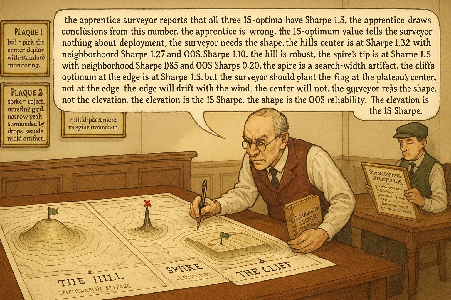
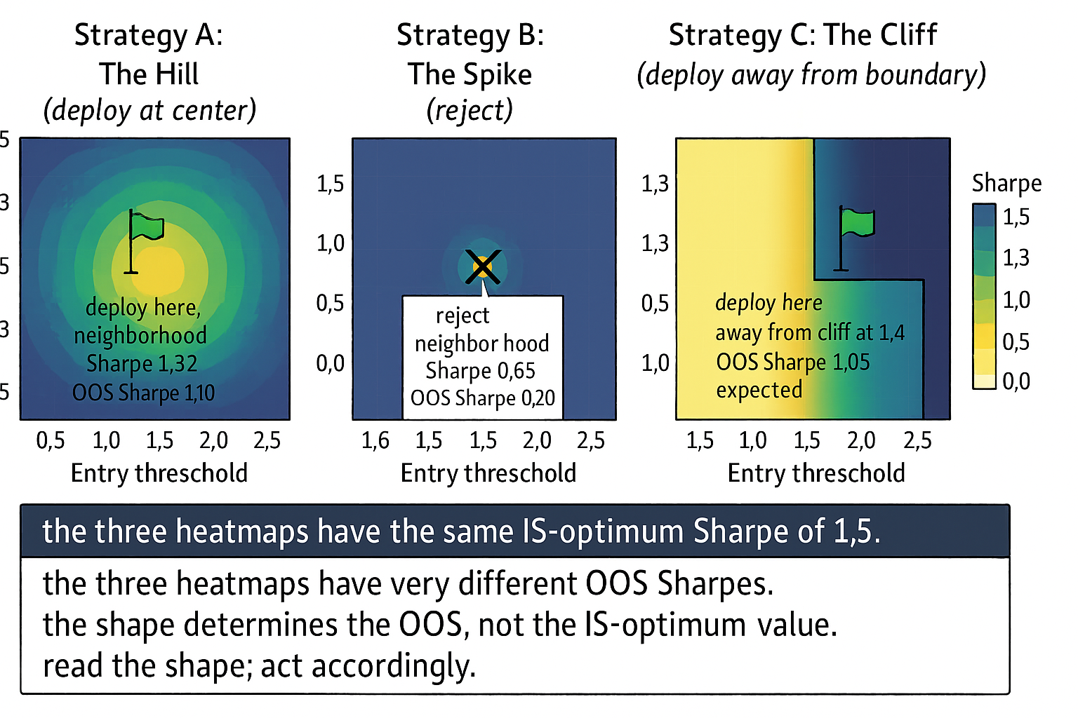
Three strategies are presented to a research review committee. Each has been optimized over the same 2-parameter grid (entry threshold, exit threshold), and each has produced an IS-optimal Sharpe of 1.5. The committee asks for the parameter-stability map of each, plotted as a heatmap of IS Sharpe over the two-parameter grid. The three heatmaps look very different.

Strategy A's heatmap shows a single broad bright region centered at the IS-optimal point, with Sharpes above 1.3 across an area of approximately 30% of the grid and Sharpes above 1.0 across approximately 60% of the grid. The contour lines around the IS-optimum are widely spaced. The shape is a hill: a robust, gently-sloped maximum.

Strategy B's heatmap shows a small bright pixel at the IS-optimal point with Sharpe 1.5, surrounded immediately by pixels with Sharpes around 0.7 to 0.9. The contour lines around the IS-optimum are tightly packed. The bright region is one or two grid cells wide. The shape is a spike: a sharp narrow peak.

Strategy C's heatmap shows a bright region with Sharpes above 1.3 occupying approximately 25% of the grid, but the bright region ends abruptly at a sharp boundary. On one side of the boundary the Sharpe is 1.4. On the other side it drops to -0.3 within one or two grid cells. The IS-optimal point is near the boundary. The shape is a cliff: a flat plateau adjacent to a sharp regime transition.

The article "Parameter Stability Beats Best Parameter" gave the discipline of choosing the plateau center. This article gives the visual taxonomy of the three common surface shapes (and a few variants), what each implies about the strategy's mechanism, and the operational response to each. The taxonomy is the diagnostic toolkit; the strategy is deployable, fragile, or regime-conditional depending on which shape its surface displays.

The hill

Operational definition. A region where the Sharpe is high relative to the surrounding grid, with gentle gradients in all directions, and the local maximum is approximately at the center of the region.

The hill shape, in operational terms. The strategy has a true Sharpe approximately equal to the hill's mean Sharpe (slightly below the peak Sharpe due to mild noise). The IS-optimum is the maximum of the hill, but parameters near the hill center produce similar Sharpes. The strategy is robust to parameter perturbation because the gentle gradient means small parameter shifts produce small Sharpe shifts.

Operational response. Choose the parameter at the hill's center, not at the IS-optimum. The center parameter has slightly lower IS Sharpe and a much wider robust neighborhood. The deployment expectation is that OOS Sharpe will be approximately 80-95% of the chosen-parameter IS Sharpe (a small gap, mostly due to general OOS noise rather than parameter fragility).

Diagnostic numbers. For a hill, the neighborhood Sharpe (across +/-25% perturbation in each parameter) is at least 80% of the peak Sharpe. The standard deviation of Sharpes across the neighborhood is small (less than 0.15 in absolute terms for a peak Sharpe of approximately 1.0). Perturbing the chosen parameter by +/-25% in any direction changes the Sharpe by less than 15%.

Examples. The classic 12-1 momentum factor on equity indices produces a hill. The classic 22-day vol-targeting on G10 FX produces a hill. The 5-day mean reversion on equity intraday produces a hill within a defined parameter range.

The spike

Operational definition. A region where the Sharpe is high at one or two grid cells and drops by more than 30% within one grid step in all directions.

The spike shape, in operational terms. The IS-optimum is a peak constructed from a small number of favorable trades that happened to cluster at this specific parameter set. The peak is a search-width artifact; the underlying strategy does not have a true Sharpe at this peak level. Small drifts in the underlying market dynamics will move the strategy off the spike, and the realized Sharpe will be far below the peak.

Operational response. Reject the spike-shaped optimum. There is no plateau to fall back to; the strategy as configured is a search-width artifact. Either the strategy specification is noise-fitting by design (drop it) or the parameter grid is too coarse to reveal a real plateau (refine the grid). Re-running with a finer grid and re-mapping the surface is the right next step; only deploying if a hill emerges at finer resolution.

Diagnostic numbers. For a spike, the neighborhood Sharpe is less than 50% of the peak Sharpe. The standard deviation of Sharpes across the neighborhood is large (greater than 0.30 for a peak Sharpe of approximately 1.0). Perturbing the chosen parameter by +/-25% drops the Sharpe by more than 40%.

Examples. Most "discoveries" from random parameter searches with k_eff in the thousands or higher produce spikes. The "amazing strategy" found via grid search on a small backtest is almost always a spike. ML-driven strategies without explicit regularization commonly produce spike-shaped surfaces.

The cliff

Operational definition. A region where the Sharpe is high across a substantial area but ends abruptly at a sharp boundary, with the IS-optimum at or near the boundary.

The cliff shape, in operational terms. The strategy is effective in the high-Sharpe region and ineffective (or actively losing) on the other side of the boundary. The boundary represents a regime transition: a parameter range where the strategy switches from working to not working, often abruptly. Examples of regime transitions:

Regime 1: trend vs mean-reversion. A strategy with very short lookback (e.g., 1-3 days) may be a mean-reversion strategy on a market and produce positive Sharpe; the same strategy at slightly longer lookback (e.g., 5-7 days) on the same market may flip to trend-following character and produce negative or zero Sharpe. The cliff is at the lookback that crosses the autocorrelation sign change.

Regime 2: position-cap binding. A strategy with low position cap may be effective; the same strategy with higher position cap may concentrate risk during regime breaks and produce negative skew. The cliff is at the position-cap level where the concentrated-risk events start to dominate.

Regime 3: cost crossing. A strategy that trades frequently may be profitable below a certain trade-frequency threshold (transaction costs are tolerable) and unprofitable above (costs swamp signal). The cliff is at the trade frequency where costs cross signal.

Operational response. Choose a parameter set well away from the cliff (toward the center of the high-Sharpe region) rather than at the IS-optimum near the boundary. The IS-optimum near the cliff has the highest IS Sharpe but the highest risk of crossing the boundary under regime drift. The center-of-region parameter has slightly lower IS Sharpe but is far from the boundary and survives regime perturbations.

Diagnostic numbers. For a cliff, the neighborhood Sharpe in the direction away from the cliff is at least 80% of the peak; the neighborhood Sharpe in the direction toward the cliff drops by more than 50%. The asymmetry is the cliff signature. The article "Slow Wandering: The Most Dangerous Type of Market Change" framed the regime-drift problem; a cliff-positioned parameter is precisely the configuration most vulnerable to slow regime drift.

Examples. Strategies whose lookback crosses the autocorrelation-sign transition. Strategies whose volatility threshold sits at the boundary between vol regimes. Strategies whose cost assumption crosses the break-even line.

Three less common surface shapes

Variant 1: the saddle. A surface with a saddle point: high in two directions and low in two others. The IS-optimum at a saddle is unstable in the directions where the Sharpe drops. Treat saddles like cliffs in the directions of decline.

Variant 2: the maze. A surface with multiple disconnected high-Sharpe regions separated by valleys. Each region may correspond to a different regime where the strategy works for a different reason. A maze surface suggests the strategy is several strategies overlaid; identify which region matches the deployed regime and deploy only on that.

Variant 3: the slope. A surface with no clear maximum, only a monotonic increase or decrease toward a boundary of the search range. The IS-optimum is at the boundary. The slope is a sign that the search range was insufficient; extend the range until the surface peaks within the searched region.

Diagnostic protocol

Five-step procedure for reading any optimization surface.

Step 1: visualize the surface. For 2 parameters, heatmap or contour. For 3+ parameters, show pairwise marginal heatmaps with other parameters fixed at the candidate plateau center.

Step 2: identify the IS-optimum and mark it. The IS-optimum is one specific point on the surface. Mark it as a starting reference.

Step 3: characterize the surrounding region. Compute neighborhood Sharpe (mean of Sharpes within +/-25% perturbation in each parameter). Compute neighborhood standard deviation. Compute gradient (rate of change of Sharpe near the IS-optimum).

Step 4: classify by shape. Hill = high neighborhood mean, low neighborhood SD, gentle gradient. Spike = low neighborhood mean, high neighborhood SD, steep gradient. Cliff = high neighborhood mean in one direction, low in the opposite direction (asymmetric gradient).

Step 5: choose action by shape. Hill = pick the center, deploy. Spike = reject or refine grid. Cliff = pick a parameter away from the cliff, toward the center of the high-Sharpe region. Deploy with regime monitoring.

The math of why shapes predict OOS

A simple model. Let SR_true(theta) be the true Sharpe surface and IS_Sharpe(theta) be the IS estimate. The IS estimate equals the true Sharpe plus mean-zero noise with magnitude depending on the per-cell sample size. The shape of the IS surface reflects the shape of the true surface plus the noise's contribution.

$$ \widehat{\text{SR}}_{\text{IS}}(\theta) = \text{SR}_{\text{true}}(\theta) + \varepsilon(\theta) $$

For a hill (broad smooth true surface), the noise contribution is small relative to the true surface, and the IS shape closely matches the true shape. The IS-optimum is a few percent above the hill's true Sharpe, and OOS realizations track. For a spike (no true Sharpe at the location, only noise), the spike is the maximum of the noise field over k_eff comparisons, and the OOS realization (drawn from the true Sharpe at that location, which is approximately zero) is far below. For a cliff (true Sharpe surface has a regime transition), small drifts in regime move the cliff location, and a parameter at the cliff edge is most sensitive to the drift.

Anti-patterns

Five mistakes specific to surface reading.

Anti-pattern 1: not plotting the surface. Skipping the visualization is the most common mistake. Without the surface map, hills, spikes, and cliffs are indistinguishable. The map is the minimum required diagnostic.

Anti-pattern 2: trusting the IS-optimum on a spike-shaped surface. The spike's IS Sharpe is a search-width artifact. Deploying the spike's parameter is deploying noise.

Anti-pattern 3: deploying at the cliff edge. The IS-optimum at the cliff has the highest IS Sharpe but the worst regime-drift sensitivity. Move toward the center of the high-Sharpe region.

Anti-pattern 4: refining the grid only at the optimum. Refinement should cover the full neighborhood to confirm the shape. Refining only at the optimum cannot distinguish a spike (whose surrounding cells remain low) from a hill (whose surrounding cells remain high).

Anti-pattern 5: not re-mapping the surface periodically. Surface shapes can change over time as the underlying dynamics drift. A strategy that was on a hill in 2015 may be on a cliff in 2024. Re-map at the same cadence as walk-forward validation.

Decision matrix

Surface shape	Neighborhood diagnostic	Deployment action
Hill	High mean, low variance, gentle gradient	Pick the center, deploy with standard monitoring
Spike	Low mean, high variance, steep gradient	Reject or refine grid
Cliff	High mean one side, low other side, asymmetric gradient	Pick parameter away from cliff, deploy with regime monitoring
Saddle	Mixed: high in some directions, low in others	Treat as cliff in the decline directions
Maze	Multiple disconnected high-Sharpe regions	Match region to deployed regime, ignore others
Slope	Monotonic toward boundary of search	Extend search range, re-map
No surface map produced	Unknown, treat as worst case	Reject pending mapping

The matrix maps surface shape to action. The pattern: produce the surface map, classify the shape, act accordingly.

Visualizing the three shapes

KEY POINTS

Optimization surfaces fall into three common shapes: hill (broad, gentle gradient, robust), spike (narrow peak, surrounded by drops, search-width artifact), cliff (wide region ending at a sharp boundary, regime transition).
Hill shape: pick the center, deploy with standard monitoring. The IS-optimum is approximately at the hill's center; the neighborhood Sharpe is at least 80% of peak; perturbations of +/-25% drop Sharpe by less than 15%.
Spike shape: reject or refine the grid. The neighborhood Sharpe is less than 50% of peak; perturbations drop Sharpe by more than 40%; the spike is a search-width artifact with no true Sharpe at the location.
Cliff shape: choose a parameter away from the boundary, toward the center of the high-Sharpe region. The neighborhood Sharpe is asymmetric: high in the direction away from the cliff, low toward it. The cliff is most vulnerable to slow regime drift.
Three less common shapes: saddle (high in some directions, low in others; treat as cliff in the decline directions), maze (multiple disconnected high-Sharpe regions, often regime-specific; match region to deployed regime), slope (monotonic toward boundary, signals insufficient search range; extend the range and re-map).
Five-step diagnostic protocol: visualize the surface, mark the IS-optimum, characterize the surrounding region (neighborhood Sharpe, SD, gradient), classify by shape, choose action by shape.
The IS Sharpe at the optimum tells you nothing about deployment without the surface shape. Three strategies with the same IS Sharpe of 1.5 may have OOS Sharpes of 1.10 (hill), 0.20 (spike), or 1.05 if positioned correctly off the cliff (cliff).
Anti-pattern: not plotting the surface. Without the visualization, all three shapes are indistinguishable.
Anti-pattern: trusting the IS-optimum on a spike. The spike's Sharpe is noise; deploying the spike's parameter deploys noise.
Anti-pattern: deploying at the cliff edge. Move toward the center of the high-Sharpe region.
Anti-pattern: refining the grid only at the optimum. Refinement should cover the full neighborhood to confirm shape.
Anti-pattern: not re-mapping the surface periodically. Shapes drift; a hill in 2015 may be a cliff in 2024.
The current article gives the visual taxonomy of optimization surfaces. The next article in the publication ("When a Stop Loss Improves Risk but Destroys Edge") begins the shift from validation discipline to specific risk-management trade-offs that show up in real strategy design.