4. Market Structure Notes June 1, 2026 8 min

4.7 How to Choose the Right Timeframe for a Strategy

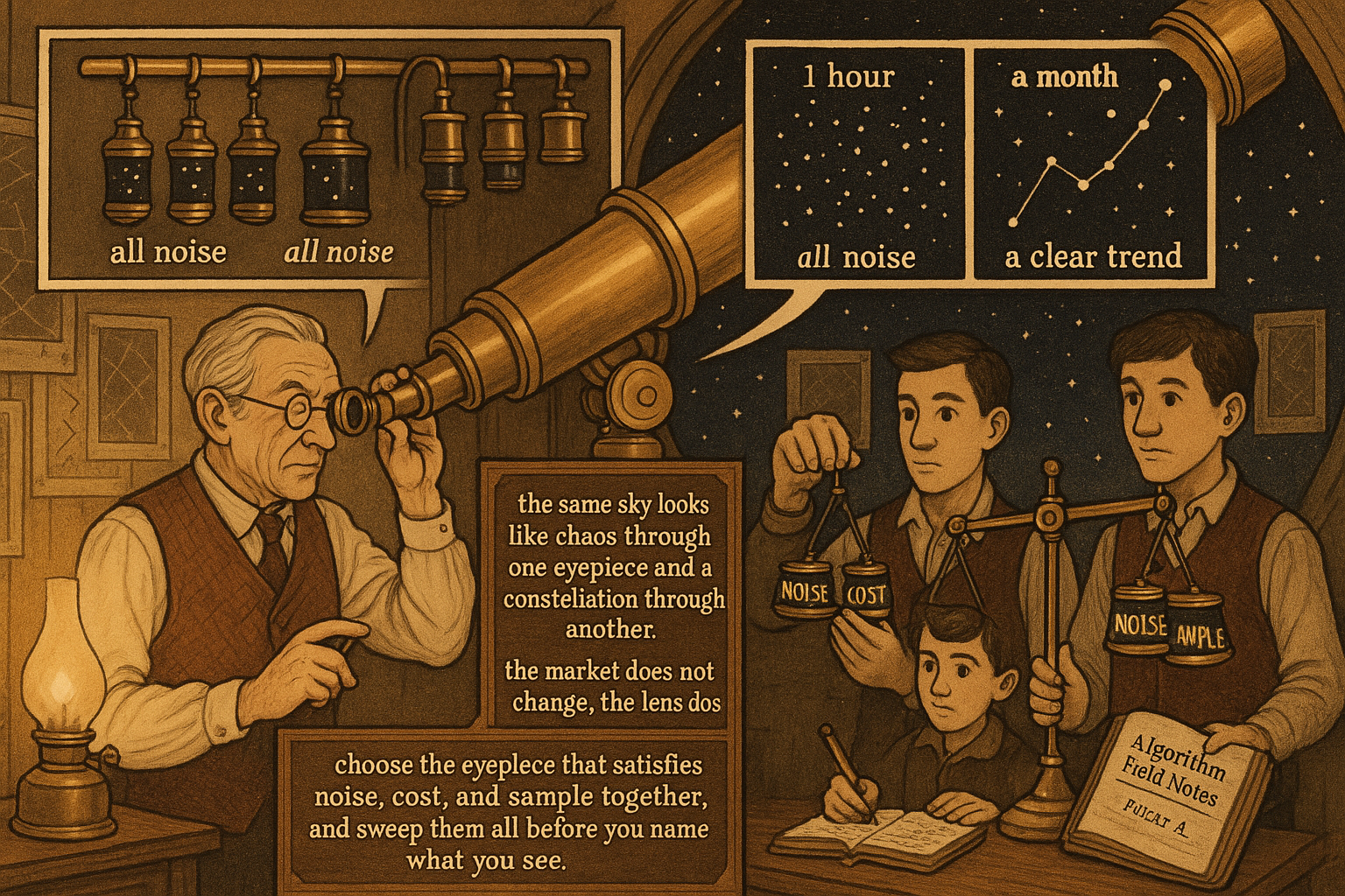
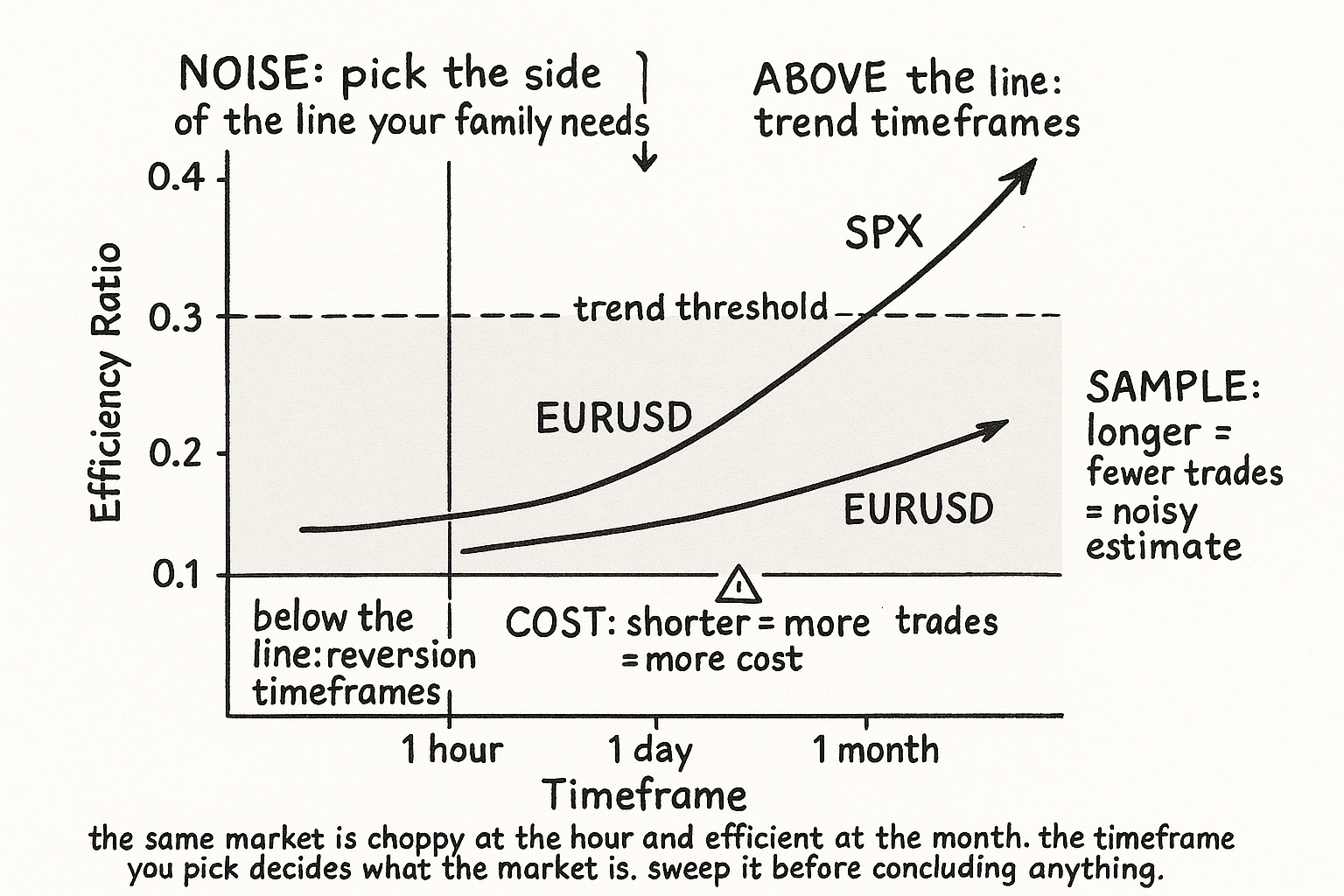
The same market is choppy at the hour and efficient at the month: the timeframe decides whether you see trend or chop. Choose it where noise, cost, and sample all hold.

Take EURUSD and compute the efficiency ratio at four timeframes on the same calendar period: hourly bars over the prior month, daily bars over the prior quarter, weekly bars over the prior two years, monthly bars over the prior decade. The readings climb as the timeframe lengthens: roughly 0.10 hourly, 0.18 daily, 0.24 weekly, 0.30 monthly. The same market is choppy at the hour and efficient at the month, because short-horizon flow mean-reverts and long-horizon flow carries a macro lean. If you build a trend system and test it on hourly EURUSD, it fails and you conclude EURUSD does not trend. If you test it on monthly EURUSD, it works and you conclude it does. Both conclusions are about the timeframe, not the market, and choosing the timeframe is therefore choosing what the market is.

This article isolates the horizon dimension that the previous articles kept flagging. "Why One Indicator Should Not Be Used on Every Market" listed the resolution horizon as one of three things that change across markets; this article makes the horizon the subject. The timeframe is not a presentation choice or a personal preference. It is the single decision that most determines whether your strategy sees trend or chop, because the noise level itself is a function of timeframe, and the article "Efficiency Ratio Explained for Traders" already showed the efficiency ratio is a curve over window length rather than a point.

The same market has different personalities at different timeframes

A market is not one thing. It is a stack of overlapping behaviors at different timescales, and which one you trade depends entirely on the timeframe you sample. The source framing is direct: long-term trends are driven by economic factors and show up on weekly and daily charts, while short-term moves are investor reactions to news and show up on high-frequency data. These are different processes generating different statistics, and a single instrument hosts all of them simultaneously.

The efficiency ratio makes this measurable. At very short timeframes (minutes, hours) almost every market is high-noise, because microstructure (bid-ask bounce, inventory management, order-flow oscillation) dominates and net direction is tiny relative to the frantic path. As the timeframe lengthens, microstructure averages out and whatever structural drift the market has begins to dominate the path, so the efficiency ratio rises. A market with real long-horizon drift (an equity index) keeps rising and becomes strongly efficient at monthly scale. A market with no drift (a range-bound currency) rises modestly and plateaus, never becoming strongly efficient at any timeframe.

The practical consequence is that the timeframe choice is upstream of the trend-versus-reversion choice from the prior articles. You do not first decide "I am a trend trader" and then pick a timeframe. The timeframe partly determines whether trend is even available. A trend strategy needs a timeframe where the efficiency ratio is high; a reversion strategy needs one where it is low; and for a given market those are different timeframes.

The three constraints that set the timeframe

The right timeframe is the one that satisfies three constraints simultaneously. Miss any one and the strategy fails for a reason that looks like a different problem.

Constraint 1: the noise constraint. The timeframe must put the efficiency ratio on the right side of your strategy's family. For a trend system, pick the timeframe where the market's efficiency ratio is highest (longer, usually) and above your trend threshold. For a reversion system, pick the timeframe where it is lowest (shorter, usually) and the microstructure mean-reversion is strongest. This is the efficiency-ratio-curve reading applied as a selection rule.

Constraint 2: the cost constraint. Shorter timeframes mean more trades, and more trades mean more round-trip costs. A signal that is profitable gross at the hourly scale can be unprofitable net because the cost-per-trade is paid hundreds of times, the exact arithmetic the article "Why Transaction Costs Should Be Added Before You Fall in Love" insisted on. The cost constraint pushes the timeframe longer; the noise constraint for a reversion system pushes it shorter. The viable timeframe is where both are satisfied, and for many reversion ideas on retail-cost instruments that window is empty, which is itself the answer.

Constraint 3: the sample constraint. Longer timeframes mean fewer independent observations in any fixed calendar history. A monthly trend system over 20 years has only 240 monthly bars and a handful of independent trades, far below the thresholds the articles "Trade-Count Thresholds for Backtest Reliability" and "Why 30 Trades Is Not a Strategy" set for a reliable backtest. The sample constraint pushes the timeframe shorter to accumulate trades, directly opposing the noise constraint for a trend system. The resolution is usually to trade a longer timeframe across a basket of markets so the trade count accumulates cross-sectionally rather than over time.

These three constraints pull in different directions, and the right timeframe is the compromise that satisfies all three at once for your specific strategy and instrument. There is no universally correct timeframe; there is the one that resolves this three-way tension for your case.

A worked timeframe selection

Suppose you want to build a trend system on EURUSD. Walk the constraints.

The noise constraint says go long: EURUSD's efficiency ratio is 0.10 hourly, 0.18 daily, 0.24 weekly, 0.30 monthly. Trend needs the ratio above roughly 0.30, so the noise constraint points at the monthly timeframe, maybe weekly.

The sample constraint pushes back hard: monthly EURUSD over 20 years is 240 bars and perhaps 15 to 25 trend trades, well under 100. That is not enough to trust, so on a single instrument the monthly timeframe fails the sample constraint.

The resolution: trade the weekly timeframe (efficiency ratio 0.24, weak but workable trend) across a basket of 8 to 12 G10 and EM currency pairs, so the trade count accumulates across markets to several hundred even though each market contributes few trades. The cost constraint is comfortable at the weekly scale because trades are infrequent and FX spreads are tight. All three constraints are satisfied: enough noise for trend (barely), enough trades cross-sectionally, low enough cost.

Now contrast a reversion system on the same EURUSD. The noise constraint points short (hourly or daily, where the efficiency ratio is lowest and reversion strongest). The sample constraint is easily satisfied because short timeframes generate many trades. The cost constraint becomes the binding one: at the hourly scale you pay the spread hundreds of times, so unless the spread is very tight relative to the reversion amplitude, the net edge vanishes. The viable timeframe is the shortest one where the average reversion still clears the round-trip cost with margin, often the daily rather than the hourly scale for retail-cost access.

The timeframe-mismatch failure that masquerades as something else

The dangerous failure is testing a strategy at the wrong timeframe and misdiagnosing the result as a different problem. Three common misdiagnoses.

Misdiagnosis 1: "this market does not trend". Often it means you tested the trend system at a timeframe where the efficiency ratio is low. The market may trend strongly at a longer timeframe you did not test. The fix is to read the efficiency-ratio curve across timeframes before concluding anything about trendability.

Misdiagnosis 2: "my reversion edge is weak". Often it means you tested at a timeframe where costs ate the edge, not where the reversion was absent. The gross edge may be strong; the net edge at that trade frequency is weak. The fix is to separate the gross signal from the cost drag and find the timeframe where the gross edge survives costs.

Misdiagnosis 3: "the strategy is unstable". Often it means you tested at a long timeframe with too few trades, so the result is sample noise the article "The Hill, the Spike, and the Cliff: Reading Optimization Surfaces" would flag as an unreliable peak. The instability is in the estimate, not the strategy. The fix is to add markets at the same timeframe to grow the cross-sectional sample.

In all three the error is the same shape: a property of the timeframe got attributed to the market or the strategy. The discipline is to hold the strategy and market fixed, sweep the timeframe, and read the efficiency ratio, the cost drag, and the trade count at each one before drawing any conclusion.

Decision summary

Strategy family	Noise constraint	Cost constraint	Sample constraint	Typical resolution
Trend / breakout	Push longer (need high ER)	Comfortable (few trades)	Push shorter (need trades)	Longer timeframe across a basket of markets
Mean reversion	Push shorter (need low ER)	Binding (many trades)	Comfortable (many trades)	Shortest timeframe where reversion clears cost
Mixed / regime-switched	Read ER curve, gate by timeframe	Moderate	Moderate	Medium timeframe with regime gate

The right timeframe is the compromise that satisfies all three constraints for your specific strategy and instrument. Sweep the timeframe and measure before concluding anything about the market.

Visualizing the timeframe-noise relationship

KEY POINTS

The timeframe is not a presentation choice; it is the decision that most determines whether your strategy sees trend or chop, because the noise level itself is a function of timeframe.
The efficiency ratio rises with timeframe: almost every market is high-noise at minutes and hours (microstructure dominates) and becomes more efficient at longer timeframes (structural drift dominates). A market with real drift keeps rising; a no-drift market plateaus.
The timeframe choice is upstream of the trend-versus-reversion choice. The timeframe partly determines whether trend is even available, so you do not pick a family first and a timeframe second.
Three constraints set the right timeframe. The noise constraint puts the efficiency ratio on the right side of your family's threshold. The cost constraint penalizes short timeframes that pay the spread many times. The sample constraint penalizes long timeframes that produce too few trades.
The three constraints pull in different directions. For a trend system, noise pushes longer and sample pushes shorter; the usual resolution is a longer timeframe across a basket of markets to accumulate trades cross-sectionally.
For a reversion system, noise pushes shorter and cost pushes back; the usual resolution is the shortest timeframe where the average reversion still clears the round-trip cost with margin.
Three misdiagnoses come from testing at the wrong timeframe: "this market does not trend" (tested where the efficiency ratio is low), "my reversion edge is weak" (tested where costs ate it), "the strategy is unstable" (tested with too few trades). Each attributes a timeframe property to the market or strategy.
The discipline: hold the strategy and market fixed, sweep the timeframe, and read the efficiency ratio, the cost drag, and the trade count at each one before drawing any conclusion.
The next article, "Price Density: A Visual Way to Measure Market Choppiness", adds a second, more visual noise measure that cross-checks the efficiency ratio and is easier to read directly off a chart.