3. Robust Systems Lab May 28, 2026 10 min

3.31 Why Transaction Costs Should Be Added Before You Fall in Love

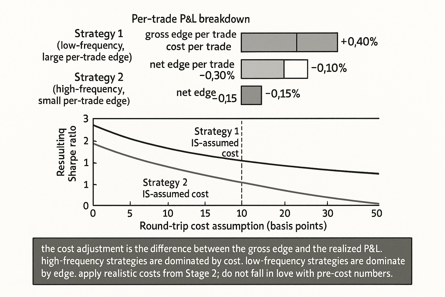
Apply realistic costs from Stage 2, not at the end. HFT strategies are cost-dominated; low-frequency edge-dominated. Teams that fall in love with pre-cost numbers resist the post-cost reality.

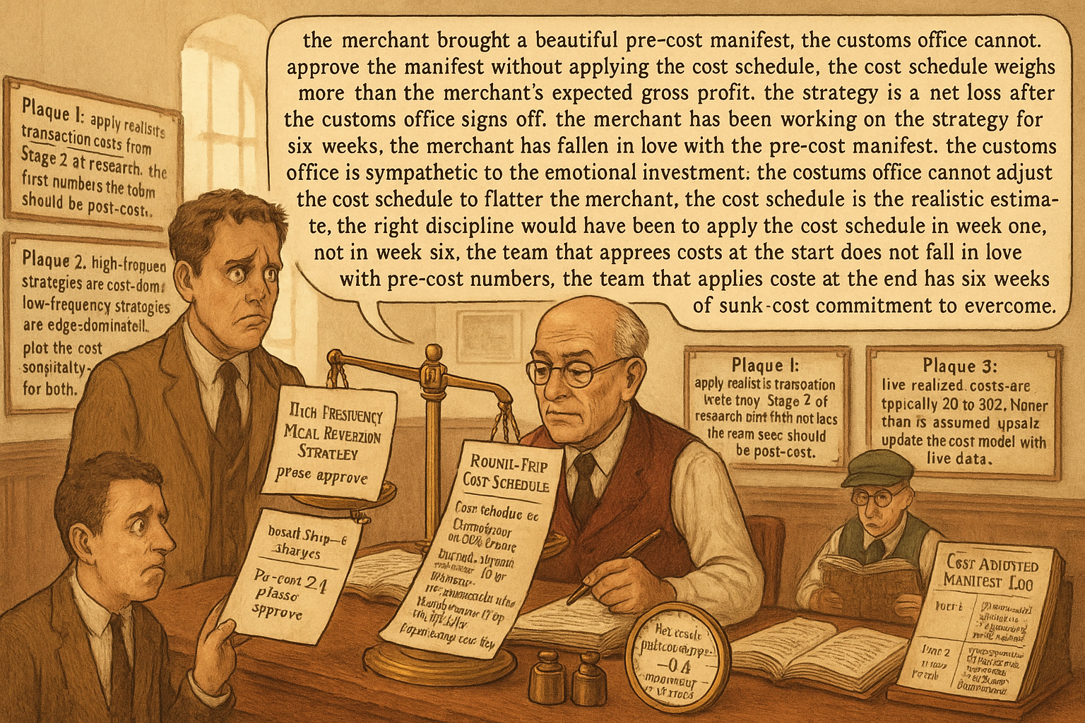
A junior researcher presents a backtest of a high-frequency mean-reversion strategy on US small-cap stocks. The IS Sharpe is 2.4 over a 3-year backtest with 18000 trades. The team is excited; the IS Sharpe is exceptional and the trade count is large enough for the result to be statistically meaningful. The team starts planning the deployment, the capital allocation, and the operational infrastructure. The senior researcher asks for the post-cost Sharpe. The junior researcher has not computed it. The team waits while the cost adjustment is applied: round-trip commission of 0.4 cents per share, average bid-ask spread of 5 cents on small-caps, slippage estimate of 1 cent on average. Total per-trade cost approximately 0.30% of the trade size. The strategy's pre-cost average win is 0.42% and average loss is -0.31%. The cost subtraction reduces both numbers symmetrically: post-cost average win 0.12%, post-cost average loss -0.61%. The post-cost expectancy is approximately -0.07% per trade. The post-cost Sharpe is approximately -0.4. The strategy is unprofitable.

The team's six weeks of excitement evaporated in the cost adjustment. The pre-cost Sharpe of 2.4 was an artifact of ignoring the cost structure of the small-cap universe. The strategy's gross signal was real (the mean-reversion pattern existed), but the gross signal was smaller than the cost overhead. The strategy was a classic "edge that exists in the data and disappears in deployment" pattern. The deployment would have produced cumulative losses approximately equal to the pre-cost cumulative profits. The team's emotional investment in the strategy had grown over the six weeks, and several team members resisted the cost-adjusted conclusion until the cost calculation was independently verified.

The discipline that prevents this pattern is procedural: apply realistic costs to the backtest before any optimization, before any pitch deck, before any team conversation about deployment. The pre-cost backtest is a tool for confirming the gross signal exists; the post-cost backtest is the deployment-relevant estimate. The team that develops emotional attachment to the pre-cost numbers has a much harder time accepting the post-cost reality. The article "How to Evaluate a Strategy Beyond Net Profit" framed the cost-related metrics in Category 7 of the evaluation panel. This article gives the procedural discipline for getting the costs right and the early-stage discipline for not falling in love with pre-cost numbers.

Cost categories to include

Five categories of trading cost, each with a typical magnitude.

Cost 1: explicit commission. The brokerage fee per trade. For US equities at retail brokers: $0 to $5 per trade. For US equities at institutional brokers: $0.001-$0.005 per share. For futures: $0.50-$3.00 per contract. For FX: 0-1 basis point. The commission is the most-often-included cost.

Cost 2: bid-ask spread. The difference between the best bid and best ask. For liquid US equities: 1-3 basis points. For mid-cap stocks: 5-15 basis points. For small-caps: 15-50 basis points. For thinly-traded stocks: 50+ basis points. For futures: 1-5 basis points on liquid contracts. For FX: 0.1-1 basis point on majors. The half-spread is typically charged on each side of a round-trip; the full spread is the round-trip cost.

Cost 3: slippage. The difference between the expected fill price and the actual fill price. Slippage depends on order size relative to liquidity, time of day, and market conditions. For small orders in liquid markets: 0.1-0.5 basis points. For larger orders: 1-10 basis points. For market-on-close orders: 5-20 basis points. For stops triggered in fast markets: 50+ basis points. The slippage estimate should be conservative; the average slippage is typically larger than the median.

Cost 4: market impact. The price movement caused by the trade itself. For small orders, market impact is approximately zero. For orders that exceed 1% of average daily volume, market impact starts to matter; for orders that exceed 5%, market impact dominates. Capacity-aware backtests include a model of market impact (often square-root or linear in trade size).

Cost 5: opportunity cost. The cost of not being filled at the desired price. Stops that are triggered intraday and not filled until close, limit orders that do not fill, partial fills, and similar issues add to the realized cost. Opportunity cost is the hardest to model and is often missed in backtests.

For a typical strategy on liquid US equities, the per-round-trip cost is approximately 5-15 basis points. For small-caps or futures, 15-30 bp. For thinly-traded instruments, 30-100 bp. The strategy's gross edge must exceed the round-trip cost times the trade frequency for the strategy to be profitable.

The math of cost-versus-edge

A simple framework. Let the gross edge per trade be E_gross and the round-trip cost be C. The net edge is:

$$ E_{\text{net}} = E_{\text{gross}} - C $$

For a strategy with gross edge 0.15% per trade (typical for a mean-reversion strategy) and cost 0.30% (typical for small-caps), the net edge is -0.15% per trade. The strategy is unprofitable, regardless of how many trades it generates or how high the Sharpe looks before costs.

The annualized return relationship. If the strategy produces N trades per year with net edge E_net per trade, the annualized return is approximately N times E_net. The cost-related sensitivity is dominated by trade frequency: a strategy that trades 100 times per year with net edge 0.5% per trade returns 50%; a strategy that trades 10000 times per year needs net edge 0.005% (0.5 basis points) per trade to return 50%. High-frequency strategies are much more cost-sensitive than low-frequency strategies because the per-trade edge they target is smaller.

$$ \text{CAGR} \approx N \cdot E_{\text{net}} = N \cdot (E_{\text{gross}} - C) $$

The discipline. Compute E_gross and C separately. Verify that E_gross > C with margin. The article "Why Profit Factor Can Lie" framed the importance of trade-level distribution; the cost adjustment applies at the trade level and propagates to all trade-level statistics.

Applying costs in a backtest

Five operational principles.

Principle 1: apply costs at the trade level, not at the aggregate level. Each trade's P&L should be reduced by the round-trip cost before computing any aggregate. Computing aggregate P&L and then subtracting cost-times-trade-count is approximately equivalent for symmetric strategies but is wrong for strategies with regime-dependent trade frequency.

Principle 2: use realistic, conservative cost estimates. The temptation is to use minimum-possible costs to flatter the strategy. The right discipline is to use realistic, slightly-conservative estimates so that surprises during deployment are upside, not downside. Conservative cost estimates: actual commission, full spread (not half), slippage estimate at the 75th percentile of historical observations, market impact for the typical order size.

Principle 3: model the cost-vs-volume relationship. Costs are not constant; they scale with order size. A strategy that works at $10M AUM may not work at $100M AUM because market impact grows. Apply the cost-versus-AUM model from the start so that capacity is visible.

Principle 4: differentiate fixed and variable costs. Per-trade commissions are fixed; spreads and slippage scale with trade size; market impact scales nonlinearly. The breakdown allows the team to understand which cost components are most damaging and how the strategy's design affects each.

Principle 5: validate the cost model against actual fills. Once the strategy has live data, compare the assumed cost structure to the actual realized costs. The actual costs are often 20-50% higher than the IS-assumed costs because the IS assumed average market conditions and live includes worst-case fills. Update the cost model with the live data.

The "fall in love" operational risk

Three psychological mechanisms.

Mechanism 1: sunk-cost commitment. The team has invested weeks on the strategy. Acknowledging the post-cost result invalidates the work. The team rationalizes alternate cost assumptions to preserve the investment.

Mechanism 2: pitch-deck momentum. The pre-cost backtest has been included in pitch decks, internal reviews, and team discussions. The team's narrative around the strategy is built on the pre-cost numbers. Reverting to post-cost requires unwinding the narrative.

Mechanism 3: comparison to competitors. The team has seen pre-cost numbers from competitors and other research and has implicitly calibrated its expectations to the pre-cost benchmark. The post-cost numbers seem disappointing relative to the pre-cost reference, even though the post-cost numbers are the operationally relevant ones.

The fix. Apply costs in Stage 2 of the research process (the prototype stage from "Optimization Comes After Testing, Not Before"). The first numbers the team sees are post-cost. The pitch deck, the internal reviews, and the team narrative are all anchored to post-cost. The pre-cost numbers are computed as a diagnostic (to verify the gross signal exists) but are not the headline.

Anti-patterns

Five mistakes specific to cost handling.

Anti-pattern 1: applying costs at the end of research. The team optimizes the strategy on pre-cost data, falls in love, then applies costs and sees a disappointing result. The right discipline is to apply costs from the start.

Anti-pattern 2: using minimum-possible cost estimates. Costs are uncertain; the IS-assumed cost is the central tendency, not the worst case. Use slightly-conservative estimates.

Anti-pattern 3: ignoring volume scaling. The strategy backtested at $1M position sizes will not have the same costs at $100M position sizes. Model market impact.

Anti-pattern 4: assuming "low-cost broker" makes the strategy profitable. The bid-ask spread and slippage do not depend on the broker; only the commission does. A strategy that requires zero commission to be profitable is a strategy that has gross edge below the spread, which is not a real edge.

Anti-pattern 5: failing to update costs with live data. Live realized costs are often 20-50% higher than IS-assumed. Update the cost model and the deployment expectation; do not assume the IS cost was accurate on the grounds that the strategy has been running.

Decision matrix

Stage of research	Right cost discipline	Wrong cost discipline
Stage 2: prototype	Apply costs from the first backtest	Defer cost analysis
Stage 3: parameter stability	Use cost-adjusted Sharpe in the surface map	Map pre-cost surface only
Stage 4: validation	Walk-forward and CSCV use cost-adjusted P&L	Validate pre-cost results
Pitch deck	Headline post-cost Sharpe; pre-cost as diagnostic	Headline pre-cost Sharpe
Internal review	All discussions use post-cost numbers	Mix pre-cost and post-cost
Capacity estimate	Model market impact at multiple AUM levels	Single-AUM cost assumption
Live deployment	Update cost model with realized fills	Assume IS cost holds
Cost validation	Compare live realized cost to IS-assumed	No cost validation

The matrix maps research stage to cost discipline. The pattern: cost discipline starts at Stage 2, not at the end. The early discipline prevents the emotional investment in pre-cost numbers.

The cost sensitivity table

A useful artifact. For the chosen strategy, compute the Sharpe at multiple cost levels:

For a hypothetical mean-reversion strategy with gross Sharpe 1.5 and IS-assumed round-trip cost 0.10%:

Round-trip cost	Resulting Sharpe	Resulting expectancy
0.05% (optimistic)	1.65	+0.20%
0.10% (IS-assumed)	1.50	+0.15%
0.15% (mildly conservative)	1.30	+0.10%
0.20% (conservative)	1.05	+0.05%
0.25% (worst-case fills)	0.75	0.00%
0.30% (small-cap-typical)	0.45	-0.05%

The table reveals the strategy's sensitivity to cost assumptions. A strategy whose Sharpe drops by 0.5+ when the cost assumption goes from 0.10% to 0.20% has substantial cost sensitivity; the deployment depends on getting the cost estimate right. A strategy whose Sharpe is stable across the range has cost-robustness.

Visualizing the cost adjustment

KEY POINTS

Apply realistic transaction costs to the backtest before any optimization, pitch deck, or team conversation about deployment. The pre-cost backtest verifies the gross signal exists; the post-cost backtest is the deployment-relevant estimate.
Five cost categories: commission (fixed per trade or per share), bid-ask spread (varies with liquidity, half-spread per side or full per round-trip), slippage (varies with order size and market conditions), market impact (nonlinear in trade size relative to ADV), opportunity cost (missed fills, partial fills, intraday-trigger-overnight-fill).
Per-round-trip cost magnitudes: liquid US equities 5-15 bp, small-caps and futures 15-30 bp, thinly-traded instruments 30-100 bp. The strategy's gross edge per trade must exceed the round-trip cost with margin.
The annualized return scales with N times net edge. High-frequency strategies are more cost-sensitive than low-frequency strategies because the per-trade edge they target is smaller. A strategy that needs 0.5 bp net edge per trade is much more cost-fragile than one that needs 50 bp.
Five operational principles: apply costs at the trade level (not aggregate), use realistic-conservative estimates, model the cost-vs-volume relationship for capacity, differentiate fixed and variable cost components, validate the cost model against actual fills.
The "fall in love" risk is psychological: sunk-cost commitment to pre-cost work, pitch-deck momentum based on pre-cost numbers, implicit calibration to pre-cost competitor benchmarks. The fix is to apply costs in Stage 2 (prototype), so the first numbers the team sees are post-cost.
The cost sensitivity table shows the Sharpe at multiple cost levels; a strategy whose Sharpe drops by 0.5+ from a 10 bp change in cost assumption is cost-fragile. Cost-robust strategies have stable Sharpes across the realistic cost range.
Anti-pattern: applying costs at the end of research. The team has fallen in love with pre-cost numbers and resists the post-cost reality.
Anti-pattern: using minimum-possible cost estimates. Use slightly-conservative estimates so deployment surprises are upside, not downside.
Anti-pattern: ignoring volume scaling. Strategy at $1M AUM has different costs than at $100M AUM. Model market impact.
Anti-pattern: assuming a low-cost broker fixes the strategy. Spread and slippage do not depend on the broker; commission does. A strategy that needs zero commission has gross edge below the spread.
Anti-pattern: failing to update costs with live data. Live realized costs are often 20-50% higher than IS-assumed. Update.
The current article gives the cost discipline. The next article in the publication ("The Backtest Integrity Checklist") gives the comprehensive procedural checklist that ensures cost handling is one of many integrity items the team verifies before deployment.