3. Robust Systems Lab May 28, 2026 9 min

3.29 Why Profit Factor Can Lie

Profit factor is dominated by extreme trades. Two strategies at PF 2.0 can have very different OOS prospects. Report trimmed PF and Gini of trade P&L alongside the headline. Don't optimize on PF.

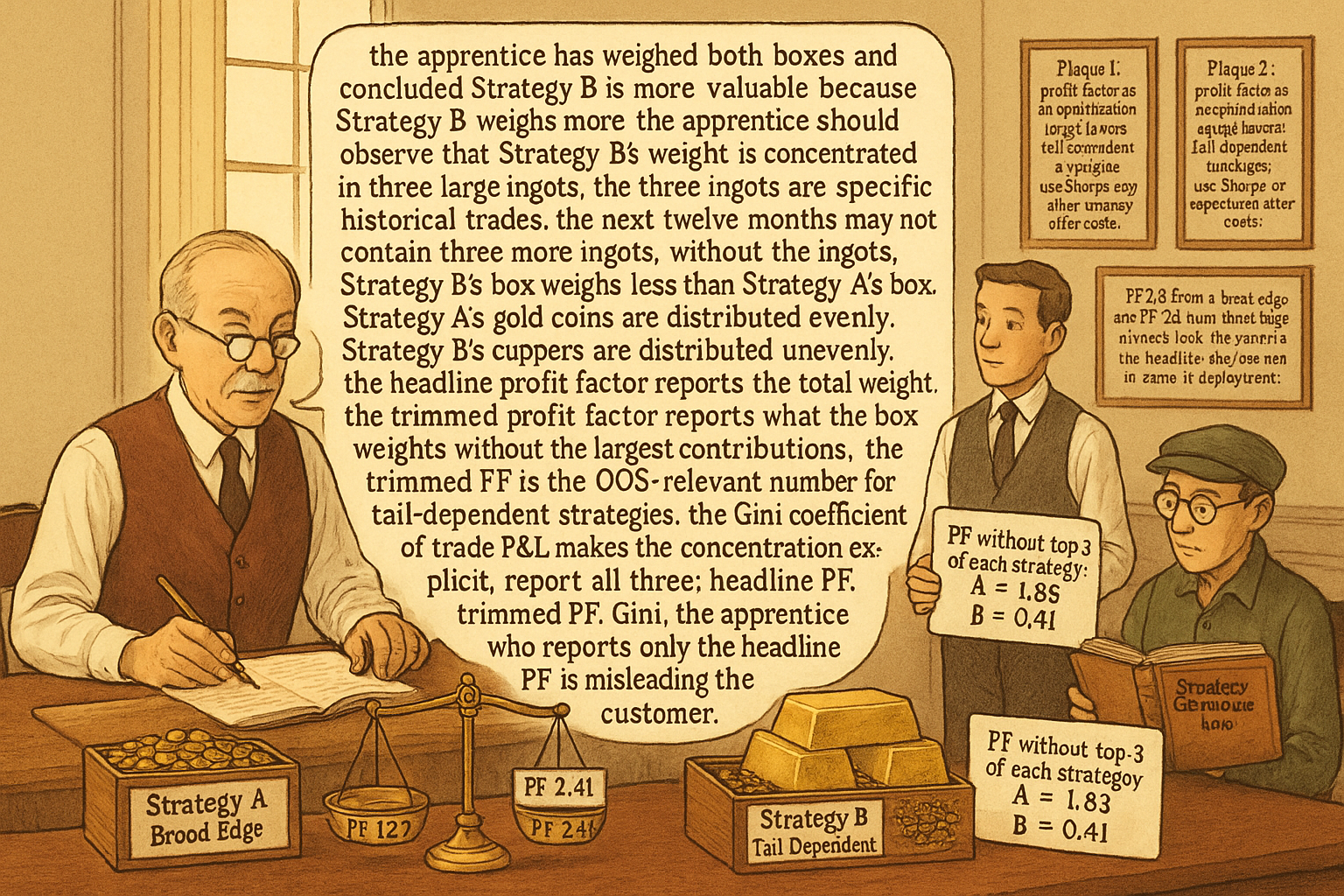
Two strategies, both with 200 trades, both with profit factor of 2.0. The pitch deck shows the profit factors and treats them as approximately equivalent in quality. They are not.

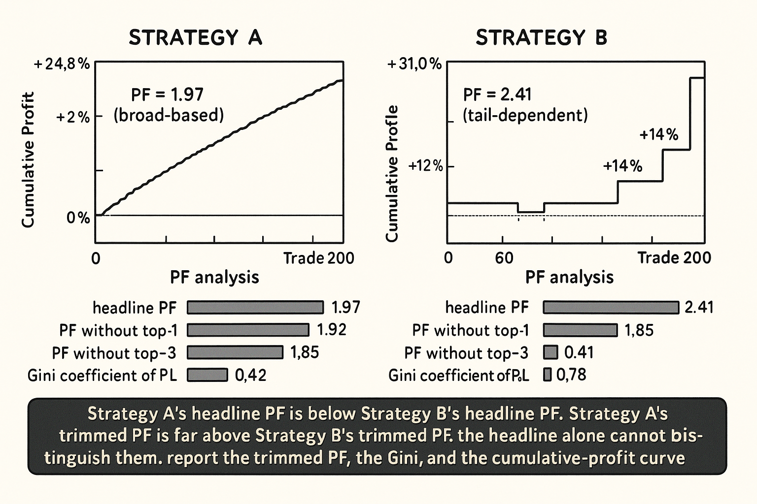
Strategy A: 120 winners averaging +0.42% each, 80 losers averaging -0.32% each. Sum of wins = +50.4%. Sum of losses = -25.6%. Profit factor = 50.4 / 25.6 = 1.97. Largest winner = +1.4%. Largest loser = -0.9%. The win and loss distributions are roughly bell-shaped with similar magnitudes. The strategy's profitability is broadly distributed across the trade history.

Strategy B: 90 winners averaging +0.10% each, 110 losers averaging -0.20% each, plus three exceptional winners of +12.0%, +14.0%, +18.0%. Sum of "regular" wins = +9.0%. Sum of three exceptional wins = +44.0%. Total wins = +53.0%. Sum of losses = 110 * 0.20 = +22.0% (in absolute value). Profit factor = 53.0 / 22.0 = 2.41. Profit factor without the three exceptional winners = 9.0 / 22.0 = 0.41 (the strategy is unprofitable on its non-exceptional trades). Largest winner = +18.0%. Largest loser = -0.6%. The strategy's profitability is concentrated in three extreme trades. The other 197 trades, in aggregate, lose money.

Strategy A's profit factor of approximately 2.0 reflects a stable, broadly-distributed edge. Strategy B's profit factor of 2.4 reflects a tail-dependent edge that depends on three specific historical trades. Strategy B's expected OOS profit factor is much lower than 2.4 because the OOS will not necessarily contain three +12% to +18% trades; if the OOS contains only "regular" trades from the underlying distribution, the OOS profit factor will be near 0.4, not 2.4. The headline profit factor numbers cannot distinguish A from B.

The article "MAE/MFE Analysis: Seeing What Net Profit Hides" framed the trade-level path information that aggregate statistics conceal. This article gives the same diagnostic for profit factor. Profit factor is one of the most-cited metrics in retail trading literature and one of the most easily manipulated. The article enumerates the failure modes, the diagnostic plots that reveal them, and the alternative metrics that complement profit factor without inheriting its weaknesses.

Profit factor, defined

The definition. Profit factor is the ratio of the sum of winning trades' P&L to the absolute value of the sum of losing trades' P&L.

$$ \text{PF} = \frac{\sum_{i: \text{P\&L}_i > 0} \text{P\&L}_i}{\sum_{i: \text{P\&L}_i < 0} |\text{P\&L}_i|} $$

A profit factor above 1 means the strategy is profitable in aggregate. A profit factor of 2.0 is often presented as a "good" threshold, with 1.5 as "acceptable" and 3.0+ as "excellent" in retail literature.

Profit factor's strengths. It is a single intuitive number that combines win rate, average win, and average loss into one ratio. It is computable from any trade record. It is invariant to the unit of position size as long as positions are sized consistently.

Profit factor's weaknesses. It is dominated by extreme outliers. It does not penalize concentration of profits in a few trades. It does not differentiate between a stable edge and a tail-dependent edge. It shows high sensitivity to the IS sample's specific outliers.

Three failure modes of profit factor

Failure 1: outlier dominance. As in the Strategy B example, a few extreme winners can dominate the numerator. The profit factor reports the aggregate ratio without indicating that the aggregate is concentrated. Removing the top 1-3 trades and recomputing the profit factor reveals the dependence; for many strategies the "trimmed" profit factor is 30-70% lower than the headline.

Failure 2: optimization gaming. A team optimizing on profit factor will produce strategies with high profit factors but potentially low Sharpe and high concentration. Profit factor rewards low-frequency strategies that catch occasional large moves; it does not reward strategies with consistent moderate edge. The optimization-target choice has structural consequences.

Failure 3: instability across samples. Because profit factor is dominated by outliers, the profit factor on different IS sub-samples can vary across a wide range. A strategy with profit factor 2.0 on a 5-year sample may have profit factor 1.4 on years 1-2.5 and 2.6 on years 2.5-5. Bootstrap or sub-sample analysis reveals the instability; the headline does not.

Diagnostic plots and statistics

Five diagnostics that complement the headline profit factor.

Diagnostic 1: cumulative profit factor curve. Plot the running profit factor as trades accumulate from 1 to N. A stable strategy shows the curve converging to a steady value. A tail-dependent strategy shows the curve jumping at specific trades and otherwise drifting. The convergence pattern is informative.

Diagnostic 2: profit factor minus top-K. Compute the profit factor with the top 1, top 3, top 5, top 10 winners removed. For a stable strategy, removing the top trades reduces profit factor by 5-15% per trade removed. For a concentrated strategy, removing the top 1 trade can drop profit factor by 30%+ and removing the top 3 can drop it by 50%+ or convert profitability to unprofitability. The "top-K-trimmed" profit factor is the operationally relevant number.

Diagnostic 3: Gini coefficient of trade P&L. The Gini coefficient measures concentration. A Gini near 0 means the P&L is evenly distributed across trades; a Gini near 1 means concentrated in a few trades. Trading strategies typically have Gini between 0.4 and 0.8; values above 0.75 are red flags for tail-dependence.

Diagnostic 4: distribution of wins and losses on log scale. The log-scale histogram reveals the shape of the win and loss distributions. A roughly normal-shaped distribution means most trades are in a typical range. A heavy-right-tailed win distribution means a few extreme trades dominate. Visualization reveals what the headline profit factor hides.

Diagnostic 5: bootstrap of profit factor. The bootstrap distribution of profit factor (covered in "Monte Carlo for Trading Systems") reveals the sampling-distribution variability. A stable strategy has a tight bootstrap distribution. A concentrated strategy has a wide distribution with a long left tail (when the bootstrap omits the extreme trades, the profit factor drops by 40-60% or more).

Operational interpretation

Three rules of thumb.

Rule 1: report profit factor with the top-3-trimmed profit factor. The two numbers together reveal whether the headline depends on outliers. If trimming the top 3 trades drops the profit factor by less than 30%, the strategy has a broad-based edge. If trimming drops the profit factor by more than 50%, the strategy is concentrated.

Rule 2: report profit factor alongside Sharpe and expectancy. A high profit factor with low Sharpe is suspicious (it suggests rare large winners with high variance). A high profit factor with high Sharpe is more credible. The combination is more informative than either metric alone.

Rule 3: do not optimize on profit factor. Optimization on profit factor produces tail-dependent strategies. Optimize on Sharpe (which penalizes variance), expectancy after costs (which penalizes high frequency), or a combined objective that includes a concentration penalty.

Cases where profit factor is informative

Three cases where profit factor is a useful diagnostic.

Case 1: small-trade strategies where outliers are clipped. For strategies with explicit position caps and small per-trade size, the trade distribution has bounded outliers. Profit factor is approximately the ratio of average win to average loss times the win rate ratio, and it is informative.

Case 2: trend-following with explicit catastrophic-loss protection. Trend followers expect a few large winners and many small losers. The profit factor of approximately 1.5-2.0 from such strategies is consistent with the structural mechanism. The catastrophic-loss protection (covered in "When a Stop Loss Improves Risk but Destroys Edge") bounds the loss-side outliers.

Case 3: high-frequency strategies with thousands of trades. With N greater than 5000, the law-of-large-numbers convergence makes profit factor a reasonably stable estimate (though still subject to outlier dominance if the underlying distribution is heavy-tailed).

Anti-patterns

Five mistakes specific to profit factor.

Anti-pattern 1: comparing two strategies on profit factor alone. Two strategies with the same profit factor can have very different OOS expected performance. Always pair with Sharpe, expectancy after costs, and the trimmed profit factor.

Anti-pattern 2: using profit factor as the optimization target. The optimization will favor tail-dependent strategies. Use Sharpe or expectancy after costs as the optimization target, with profit factor as a secondary diagnostic.

Anti-pattern 3: reporting only the headline profit factor without the trimmed values. The dependence on top trades is invisible without the trimmed metric. The dependence is the operationally relevant information.

Anti-pattern 4: applying the "PF > 2.0 is good" threshold uniformly across strategy families. Trend-following strategies typically have PF approximately 1.4-1.8 (many small losers, few large winners) and are deployable. Mean-reversion strategies typically have PF approximately 1.6-2.5 (many small winners, few medium losers) and are deployable. The threshold depends on the family.

Anti-pattern 5: confusing PF stability with strategy stability. A strategy whose PF is stable across IS sub-samples may still have other instabilities (regime sensitivity, parameter fragility, decay over time). Combine PF stability with the diagnostics from "Walk-Forward Testing" and "Parameter Stability Beats Best Parameter".

Decision matrix

Profit factor pattern	Interpretation	Action
Headline PF 2.0, trimmed-top-3 PF 1.7	Stable broad-based edge	Treat as informative
Headline PF 2.4, trimmed-top-3 PF 0.8	Tail-dependent edge	Investigate; do not trust headline
PF 2.0 with high Sharpe (>1.0)	Stable edge with low variance	Strong combination
PF 2.0 with low Sharpe (<0.5)	Outlier-dependent	Investigate the outliers
Cumulative PF curve smoothly converges	Stable	Trust
Cumulative PF curve jumps at specific trades	Concentrated	Investigate the jumps
Gini coefficient of trade P&L > 0.75	High concentration	Red flag
Gini coefficient < 0.55	Low concentration	Stable
Bootstrap PF distribution is wide	Sampling instability	Larger sample needed
Bootstrap PF distribution is tight	Stable	Trust
PF used as optimization target	Tail-dependent strategies result	Switch to Sharpe target

The matrix maps profit-factor pattern to action. The pattern: profit factor is one diagnostic; combine with concentration measures, Sharpe, and bootstrap analysis.

Visualizing profit factor's lie

KEY POINTS

Profit factor is the ratio of sum of winning trades to absolute sum of losing trades. PF > 1 means profitable in aggregate; "good" thresholds in retail literature are 1.5-3.0 depending on the strategy family.
Three failure modes: outlier dominance (a few extreme trades inflate the ratio), optimization gaming (optimizing on PF produces tail-dependent strategies), instability across samples (PF varies across a wide range over IS sub-samples for concentrated strategies).
Two strategies with the same headline PF can have very different OOS expectations. A stable broad-based PF 2.0 strategy is approximately as profitable OOS. A tail-dependent PF 2.4 strategy that depends on three large winners may have OOS PF near 0.4 if the OOS does not contain comparable outlier trades.
Five complementary diagnostics: cumulative PF curve (stable strategy converges smoothly), PF minus top-K (trimmed PF reveals concentration), Gini coefficient of trade P&L (concentration index), distribution of wins and losses on log scale (visualize the tail), bootstrap PF distribution (sampling stability).
Three operational rules: report headline PF with the top-3-trimmed PF (concentration diagnostic), report PF alongside Sharpe and expectancy (combined informativeness), do not optimize on PF (use Sharpe or expectancy after costs as optimization target).
Three cases when PF is informative: small-trade strategies with bounded outliers, trend-following with explicit catastrophic-loss protection, high-frequency strategies with thousands of trades.
The math: PF is dominated by the numerator's largest contributions and the denominator's largest contributions. A heavy-right-tailed P&L distribution produces an unstable PF. A bounded P&L distribution produces a stable PF.
Anti-pattern: comparing two strategies on PF alone. Pair with Sharpe, expectancy, trimmed PF.
Anti-pattern: using PF as the optimization target. Optimization will favor tail-dependent strategies.
Anti-pattern: reporting only headline PF without trimmed values. The concentration is invisible.
Anti-pattern: applying "PF > 2.0 is good" uniformly across families. Trend-following typically has PF 1.4-1.8 and is deployable; mean-reversion typically has PF 1.6-2.5 and is deployable.
Anti-pattern: confusing PF stability with strategy stability. Combine with parameter-stability and walk-forward diagnostics.
The current article gives the profit-factor-specific diagnostic. The next article in the publication ("How to Evaluate a Strategy Beyond Net Profit") covers the comprehensive metrics framework that uses PF as one of many complementary diagnostics rather than the headline.