The previous article showed that one backtest is one sample drawn from a distribution of possible backtests. This article goes one level deeper. Even if a researcher could run an infinite number of backtests over all of recorded market history, the conclusions would still rest on one sample, because market history itself is one trajectory through possibility space. The market plays out once. There is no second universe in which the same starting conditions produced a different sequence of price moves for comparison.

This is not a methodological issue that can be fixed with better technique. It is an epistemological limit on what any participant in a non-repeatable system can learn from observation alone.

The two-layer sampling problem

A backtest result sits inside two layers of uncertainty.

The inner layer is sampling variability within history. Given the realized price sequence of SPX from 1990 to 2024, a strategy run on that sequence produces one point estimate of its true performance. Different windows of the same sequence produce different point estimates. The block bootstrap and the standard error formulas address this layer. The previous article was about this.

The outer layer is the realized history itself. The SPX 1990 to 2024 is one possible path through the joint distribution of every variable that drives prices: monetary policy, technology adoption, demographic shifts, geopolitics, and the behavioral patterns of every trader who showed up. Under slightly different initial conditions or slightly different shocks, the realized sequence would look different. The realized history is one draw from a meta-distribution of possible histories.

A simple decomposition makes the two layers visible:

Where μ̂_backtest is the estimated edge from the backtest, μ_regime is the true edge under the current data-generating regime, ε_sampling is the inner-layer noise from finite N within history, and δ_regime drift is the outer-layer noise from the fact that the realized history is one trajectory and the regime parameters themselves shift over time.

Statistics can shrink ε_sampling toward zero with more data and better methods. Statistics cannot shrink δ_regime drift, because there is no second history to compare against.

Why physics gets away with what trading cannot

Physics solves the one-sample problem by repetition. The same experiment runs millions of times in the lab or in nature: every dropped object, every electron, every photon. The repeated trials are draws from the same underlying distribution. Sample sizes are practically infinite.

Climate science sits in a harder position. There is one Earth. Climate scientists work around this by collecting many proxies (ice cores, tree rings, ocean sediment cores), looking at other planets, and building physical models that have to match the one trajectory the planet took. Their conclusions are weaker than particle physics conclusions for exactly this reason.

Trading is even worse. There is one financial history, and that history is the output of active participants who see the data, respond to it, and change the system. Markets adapt. The data-generating process of 2024 is not the data-generating process of 1990. A strategy that worked on the older data was operating in a different statistical world. This is the non-stationarity problem and it interacts with the one-sample problem in a vicious way.

Non-stationarity makes it worse

Standard statistical inference assumes the population stays the same while different samples are drawn from it. In markets, the population drifts. Volatility regimes change. Correlations shift. Liquidity providers come and go. Interest rate regimes flip. Crowding makes formerly profitable patterns disappear.

When the population is non-stationary, a sample from one decade is not interchangeable with a sample from another decade. Pooling them increases nominal N but does not increase information about the current population. A model fit on 1980 to 2020 is fitting to multiple populations stitched together. The fit minimizes joint error across populations that no longer all exist.

The result is that effective N is much smaller than nominal N. A 30-year backtest of an equities strategy might span only two or three relevant regimes. The other 27 years are information about markets that no longer exist. That is not 30 years of evidence about today's market. That is roughly three samples of three different markets, with no guarantee any of them still applies.

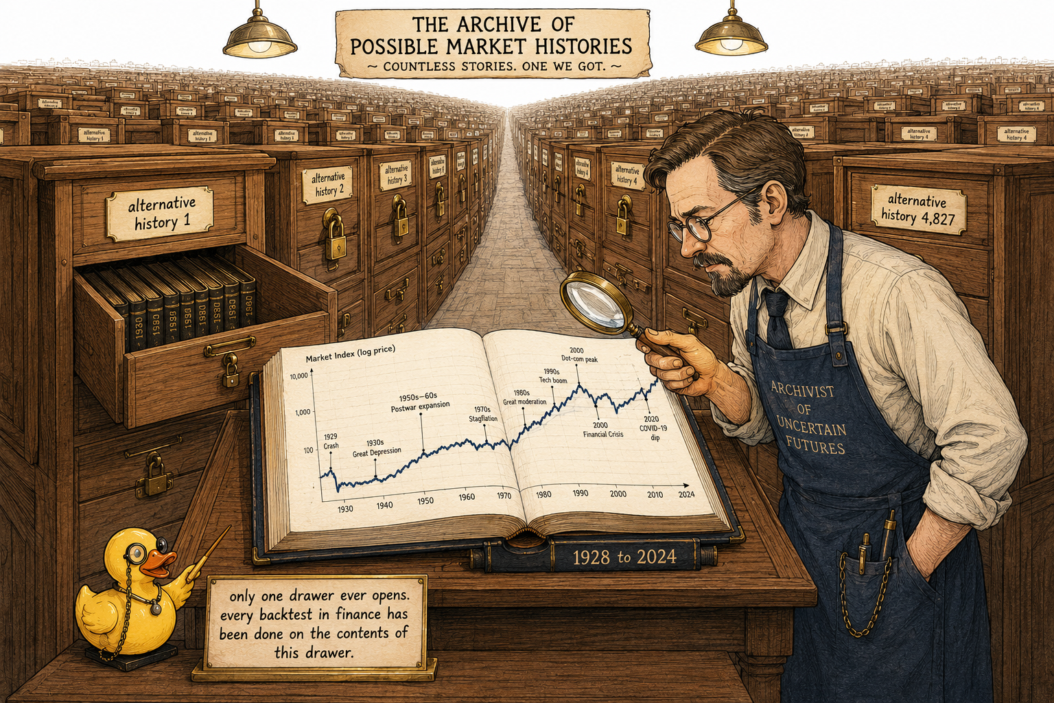
Visualizing the one-sample problem

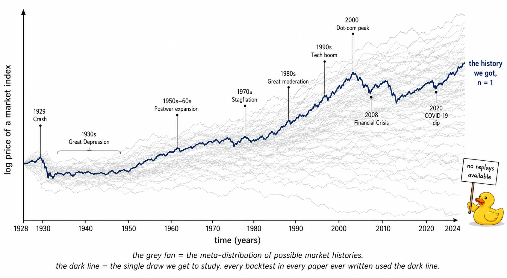
The thick navy line is the only thing any trader has ever had access to. Every formula, every backtest, every published edge was estimated on that one line. The grey fan is the world the researcher would need to see to be confident about any inference. The fan is not available.

What can be done despite the one-sample limit

Five techniques partially compensate for the missing fan. None of them solve the problem.

1. Cross-section as a sample multiplier. Instead of one market over 30 years, study 30 markets over the same window. If a rule works on equities, fixed income, FX, and commodities simultaneously, the evidence is stronger than if it works on equities alone. The instruments are not independent samples, but their idiosyncratic noise is partly independent, so the joint test is more demanding than any single one.
2. Cross-period replication. Split history into non-overlapping windows large enough to span at least one economic cycle. Estimate the rule on each window independently. Stable results across windows are evidence that the rule does not depend on the one global trajectory. Unstable results are evidence that it does.
3. Synthetic histories via simulation. Build a stochastic model of returns that respects the documented properties of markets (fat tails, volatility clustering, autocorrelation, regime switching). Generate thousands of synthetic price paths from the model. Test the rule on each. The synthetic distribution of rule outcomes substitutes for the missing meta-distribution. The substitution is imperfect because the model is wrong (always wrong, in different ways). The exercise still produces a sharper estimate than the single historical path.
4. Robust phenomena as priors. Effects that show up across centuries, across asset classes, and across countries (the value premium, the momentum effect, the volatility risk premium, the term premium) have survived many implicit out-of-sample tests. They are not guaranteed to survive the next one, but they are stronger starting points than effects that have only been observed in one market over one decade.
5. Position sizing for the larger uncertainty. The math says the standard error on any backtested edge is wider than the standard formulas suggest, because nominal N overstates effective N when history is non-stationary. The honest response is smaller positions, broader diversification, and lower expected returns than the headline backtest suggests.

The active-participant problem

There is one more wrinkle that makes financial history different from any other one-sample problem.

In physics, the experimenter does not influence the electron. In climate science, the climatologist does not influence the ice age. In markets, the participants see the published research, the backtests, and the strategies, and trade on them. Edges get crowded out. Patterns get arbitraged away. The act of discovering and publishing a pattern changes the data-generating process going forward.

This means the one realized history is not a passive sample of a fixed underlying process. It is the output of a feedback loop where participants are constantly updating their behavior based on what they think the process is. The realized path of the system is correlated with the beliefs of the participants about the path of the system.

The practical consequence is that historical evidence depreciates faster than statistical formulas suggest. The longer an edge has been known, the more it has been traded against, and the less reliable historical data on it becomes. The half-life of a published anomaly is finite and often short.

The honest statement

Every backtested edge is the edge that worked on the one history that happened. The single-sample problem does not make backtesting useless. It makes confident conclusions from any backtest, no matter how clean the methodology, dishonest.

A trader who reports a backtested Sharpe of 1.5 with the implicit claim "this is the edge of the strategy" has overstated what was learned. The accurate version is: "this is the edge of the strategy on the one history available, with methodological uncertainty captured in the confidence interval and additional uncertainty from the one-history problem captured in the priors used to interpret the confidence interval."

That sentence does not fit on a marketing slide. It is the correct sentence anyway.

KEY POINTS

• A backtest result sits inside two layers of uncertainty. Inner layer: sampling variability within history. Outer layer: history itself is one trajectory from a meta-distribution of possible histories.
• The decomposition μ̂_backtest = μ_regime + ε_sampling + δ_regime drift makes the layers explicit. Statistics can shrink ε_sampling. Statistics cannot shrink δ_regime drift.
• Physics handles the one-sample problem with repetition. Climate science handles it with proxies and physical models. Trading has neither, plus an active-participant feedback loop that changes the data-generating process while it runs.
• Non-stationarity compounds the one-sample limit. A 30-year backtest typically spans only two or three relevant regimes. Effective N is much smaller than nominal N.
• Five partial workarounds: cross-section across instruments, cross-period replication, synthetic histories via simulation, priors from effects that survive across centuries and asset classes, and position sizing that respects the larger true uncertainty.
• Edges depreciate after publication. The history that contained the edge before it was known is not the same as the future history that will contain the edge after it is traded against.
• None of these workarounds solve the problem. They tighten the inference relative to what one backtest alone provides.
• The honest statement about any backtested edge is that it is the edge that worked on the one history available. Reporting it as the edge of the strategy is overstating what was learned.