3. Robust Systems Lab May 28, 2026 11 min

3.9 When Forcing Stationarity Destroys Information

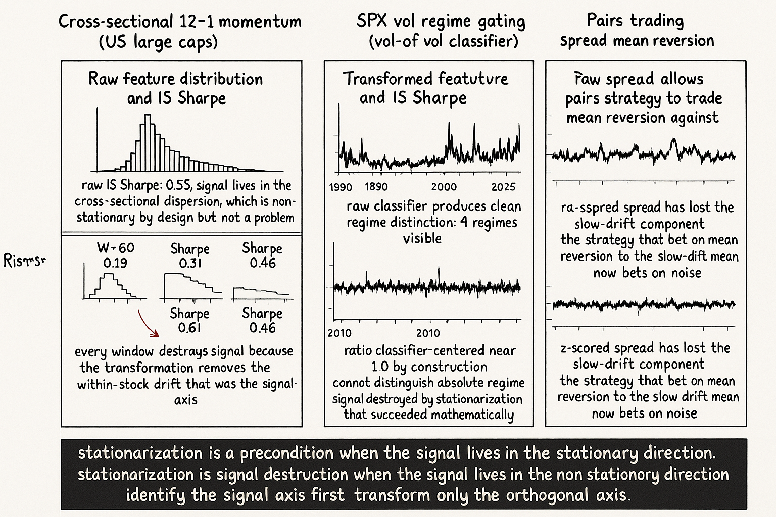
Stationarization destroys signal when the strategy lives in the non-stationary part. 12-1 momentum raw Sharpe 0.55, time-series z-scored 0.18. Find the signal axis, transform only the orthogonal one.

A researcher builds a cross-sectional momentum strategy on US large-cap equities. The signal is the 12-month total return minus the 1-month total return, ranked across the universe. The historical Sharpe of this signal in its raw form (1965 to 2024) is approximately 0.55. The researcher reads the prior article on stationarity transformations, applies a rolling 60-day z-score to each stock's 12-1 momentum series before ranking, and re-runs the backtest. The new Sharpe is 0.18. The researcher tries a 252-day z-score window. New Sharpe 0.31. The researcher tries 1000 days. Sharpe 0.46. The original raw form, with no z-scoring, beats every transformed version. The transformation pipeline that the methodology demanded was a destruction-of-signal operation, not a stationarization-of-feature operation.

The diagnosis: the 12-1 momentum signal lives in the non-stationary component of each stock's return distribution. Stocks that are in a sustained uptrend have shifted their return distribution upward; the ranking captures this shift. The rolling z-score within each stock's own history removes exactly the shift that the strategy was supposed to consume. After z-scoring, every stock looks "normal" relative to its own recent history, and the cross-sectional ranking has no information left. The transformation worked perfectly as a stationarizer (the within-stock distribution is stable across windows). The transformation also destroyed the signal.

This is the case the prior article ("How to Make Indicators More Stationary") flagged at the end. Stationarization is a precondition for reliable consumption when the strategy depends on a stable feature distribution. Stationarization is a destructive operation when the strategy depends on the non-stationary component of the feature itself. The two cases look identical until you ask the right question: what part of the feature is the strategy trading? The answer determines whether the transformation is the right tool or the wrong one. This article gives the framework for distinguishing the two cases, the diagnostic that catches over-aggressive stationarization, and the operational rule for when to leave a feature alone.

The signal-vs-stationarity dichotomy

Three categories, each with a different prescription.

Category 1: stationarity-violating noise. The non-stationary component is irrelevant to the signal the strategy consumes. Example: the absolute price level of SPX is non-stationary; a strategy designed around price-relative-to-MA consumes the deviation, with the level discarded. Stationarize aggressively (log-relative, divide by reference). The signal is preserved by the transformation; the noise (level drift) is removed.

Category 2: stationarity-violating signal. The non-stationary component is the signal. Example: the 12-1 momentum factor; the cross-sectional dispersion of multi-month returns; the long-horizon trend in interest-rate spreads. Stationarize cautiously or not at all. The transformation removes the very thing the strategy targets.

Category 3: mixed. The feature has both stationary signal and non-stationary noise components, and a stationary signal component, and a non-stationary signal component. Example: RSI on a single asset; the indicator has stable structure (the bounded oscillator behavior) plus a slow drift in the within-bounds distribution that may or may not be signal. Apply a partial transformation that removes only the noise component, or accept some non-stationarity in the signal component.

The classification is not always obvious from the indicator definition. The right question to ask: is the strategy trading the absolute level of this feature, or the relative position of this feature against its own history, or the cross-sectional rank of this feature against other instruments? Each answer points to a different transformation strategy.

The information-loss test

A diagnostic that catches over-aggressive transformation. Compute the mutual information between the raw feature and the target return, and between the transformed feature and the target return. The ratio gives the fraction of predictive information preserved by the transformation.

$$ \text{Information retention} = \frac{I(\tilde{X}; Y)}{I(X; Y)} $$

A retention near 1.0 means the transformation kept the signal. A retention well below 1.0 (say, under 0.6) means the transformation removed signal. A retention near 0 means the transformation removed the signal. The article "Relative Entropy as an Indicator Quality Score" framed the information-theoretic measurement at the indicator-quality level; the same machinery applies here at the transformation-evaluation level.

In practice, mutual information estimation needs care: it is sensitive to binning, sample size, and the joint distribution's tail behavior. A simpler proxy: compute the IS Sharpe of the strategy with raw feature and with transformed feature on the same window. If the transformed-feature Sharpe is materially lower than the raw-feature Sharpe, the transformation destroyed signal. The 12-1 momentum example at the top of this article is a clean case: raw Sharpe 0.55, z-scored Sharpe 0.18 to 0.46 depending on window. The transformation cost most of the signal.

Specific cases where stationarization destroys signal

Five common patterns.

Pattern 1: differencing a trending price for a trend-following strategy. The strategy targets the trend, which is the non-stationary component of the price. Differencing converts price to returns, which are approximately stationary. The strategy now consumes a feature with no trend information. The trend strategy on differenced returns has near-zero Sharpe by construction.

Pattern 2: rolling z-scoring a long-horizon momentum factor. The example at the top of this article. The strategy targets the cross-sectional difference in long-horizon momentum, which lives in the non-stationary mean-shift of each stock's distribution. Rolling z-score within each stock removes the shift. The transformation works as stationarizer and as signal destroyer simultaneously.

Pattern 3: dividing a regime indicator by its own moving average. A vol-regime classifier is built to detect when current vol is high relative to long-run vol. Dividing current vol by its own rolling average creates a ratio that is approximately stationary by construction (the long-run mean of the ratio is approximately 1.0). The ratio has no information about the absolute regime; a 30%-vol regime and a 12%-vol regime can both have ratio 1.0. The vol-regime gate that consumes the ratio cannot distinguish high-vol from low-vol in absolute terms.

Pattern 4: ranking a long-horizon trend within a too-short window. A multi-year trend signal is ranked within a 60-day rolling window. The 60-day rolling rank has no memory of the multi-year trend; every observation is in the same rolling distribution as the recent observations only. The trend strategy that consumed the rank has lost the long-horizon information.

Pattern 5: applying GARCH-residualization to remove all heteroskedasticity. A strategy that consumes the volatility regime as its signal will be devastated by GARCH-residualization, which removes precisely the heteroskedasticity that the strategy wanted. The residual feature is approximately Gaussian and approximately stationary; it is also approximately useless for the original strategy.

The pattern across the five: the transformation removes the same component of the feature that the strategy depends on. The transformation is technically correct as stationarization but operationally wrong because it does not preserve the signal.

The right framework

Three principles for deciding when to stationarize.

Principle 1: identify the signal axis before applying any transformation. The signal axis is the variable that the strategy depends on for its edge: the cross-sectional rank, the within-asset deviation, the absolute level, the rate of change, the regime category. The transformation must preserve the signal axis. If the transformation eats the signal axis, do not apply it.

Principle 2: stationarize in the orthogonal direction. If the signal is in the cross-sectional dimension, stationarize each instrument's time series so the cross-section is comparable but the within-instrument signal is preserved. If the signal is in the time-series dimension, stationarize the cross-section so the within-asset signal is preserved. The two transformations are orthogonal in their stationarization-vs-signal trade-off.

Principle 3: accept some non-stationarity in the signal direction. The strategy is robust to feature non-stationarity in the direction the signal lives, because the strategy was built to consume that non-stationarity. Trying to "fix" the non-stationarity in that direction destroys the strategy. The right discipline is the regime-coverage discipline (covered in "Regime Coverage: Why Your Backtest Needs Different Market States" later in this pillar): make sure the backtest covers enough regimes that the signal is validated across the non-stationary component the strategy needs.

A worked example. The cross-sectional 12-1 momentum strategy: signal axis is the cross-sectional rank of long-horizon returns. Stationarize across stocks (so a 5% return on Apple and a 5% return on a microcap are comparable in vol-adjusted terms) but do not stationarize within each stock's time series (because the within-stock drift is the signal). The right transformation: divide each stock's 12-1 return by the cross-sectional dispersion of 12-1 returns at that date, so the cross-sectional comparison is on a consistent scale, but each stock's own time series retains its trend information.

$$ \tilde{m}_t^{(i)} = \frac{m_t^{(i)} - \overline{m}_t^{(\text{cross})}}{\sigma_t^{(\text{cross})}}, \qquad m_t^{(i)} = \text{12-1 momentum of stock } i $$

The transformation is a cross-sectional z-score (each stock's momentum standardized against the cross-section at the same time), not a time-series z-score (each stock's momentum standardized against its own history). The cross-sectional version preserves the within-stock trend signal and stationarizes the cross-section.

Cases for leaving a feature raw

Three signals that argue against any transformation.

Signal 1: the raw feature already passes the stationarity diagnostics on the strategy's intended deployment regime. The rolling mean and std are stable, the histograms by window overlap, the threshold percentile is consistent. No transformation is needed.

Signal 2: the strategy's edge IS the non-stationary component, and the non-stationarity is structural rather than spurious. Trends in interest rates that reflect Fed policy are signal. Cross-sectional dispersion in earnings growth that reflects economic structure is signal. The non-stationarity in these features is the data the strategy is trying to read. Removing it removes the signal.

Signal 3: the transformation candidates fail the information-loss test. The transformed-feature Sharpe is materially lower than the raw-feature Sharpe across multiple windows and parameter choices. The transformation is destroying signal regardless of which window or parameter is chosen.

In all three cases, leave the feature alone. Apply other defenses against non-stationarity (regime-coverage backtesting, walk-forward retraining, regime-conditional gating from the prior articles in this pillar) rather than feature-level transformation.

Anti-patterns

Five mistakes specific to the over-stationarization failure mode.

Anti-pattern 1: applying every transformation in the prior article's recipe matrix without testing the information-loss. The recipe matrix gives starting points; each strategy needs verification that the transformation preserved signal. The information-loss test (or the IS-Sharpe-with-raw-vs-transformed comparison) catches the cases where the recipe was wrong for the strategy's signal axis.

Anti-pattern 2: assuming that "more stationary" is always "better". A perfectly stationary feature has no time-series structure and is uninformative for any time-dependent signal. The right amount of stationarity is the minimum needed for the strategy to consume the feature reliably, not the maximum the toolkit can produce.

Anti-pattern 3: confusing the strategy class. A strategy that trades cross-sectional rank does not need within-instrument time-series stationarity. A strategy that trades within-instrument level deviations does not need cross-sectional comparability. Applying both transformations because "we use both kinds of strategies" produces a feature that is not appropriate for either.

Anti-pattern 4: stationarizing before the diagnostic. The right order is: diagnose the violation, identify whether the violation is signal or noise, then apply the matching transformation. The wrong order is: apply the standard transformation pipeline, then diagnose the result. The wrong order makes the diagnostic conditional on the transformation, which masks signal destruction.

Anti-pattern 5: rejecting a strategy because the raw feature failed standard stationarity tests. ADF and KPSS tests on the raw 12-1 momentum factor fail because the factor is correctly non-stationary by construction (the cross-sectional dispersion of multi-month returns drifts). Rejecting the strategy on the test result alone discards a real signal. The right discipline: pass the test on the cross-sectional comparability axis, accept the non-stationarity on the signal axis, validate by regime coverage instead of by feature-level test.

Decision matrix

Strategy class	Signal axis	Right stationarization	Wrong stationarization
Cross-sectional momentum	Cross-sectional rank	Cross-sectional z-score	Time-series z-score per asset
Time-series momentum	Within-asset trend	None or vol-normalize	Differencing the price
Mean reversion (within-asset)	Within-asset deviation	Rolling rank with W matched to regime	Rank with W matched to holding period
Vol-regime gating	Absolute vol level	Long-window scaling against multi-decade reference	Short-window ratio against own MA
Spread / yield-curve	Persistent drift	None or KPSS-passing differencing	Aggressive z-scoring
Volatility prediction	Vol regime + clustering	Log-vol with persistent component	GARCH-residualization to remove heteroskedasticity
Earnings surprise	Cross-sectional shock magnitude	Cross-sectional z-score	Time-series z-score per stock
Pairs trading	Within-pair spread mean reversion	Difference + rolling mean subtract on the spread	Aggressive ranking that loses the level

The matrix is operational, illustrative. Each strategy needs verification of the signal axis before any transformation choice.

Visualizing the trade-off

KEY POINTS

Stationarization is a destructive operation when the strategy depends on the non-stationary component of the feature. The cross-sectional 12-1 momentum strategy's raw Sharpe is 0.55. The same strategy after rolling-z-scoring each stock's series gives Sharpe 0.18 to 0.46 depending on window. The transformation worked as stationarizer and destroyed signal.
Three categories of feature non-stationarity: stationarity-violating noise (transform aggressively), stationarity-violating signal (do not transform), mixed (partial transformation in the noise direction only).
The classification depends on the signal axis: the variable the strategy depends on for its edge. Cross-sectional rank, within-asset deviation, absolute level, rate of change, regime category. The transformation must preserve the signal axis.
The information-loss test catches over-aggressive transformation. Compare the IS Sharpe of the strategy with the raw feature versus with the transformed feature; a material drop is evidence the transformation removed signal. Mutual information ratio between transformed and raw with the target return is the formal version.
Five common patterns where stationarization destroys signal: differencing a trending price for trend-following, rolling z-scoring a long-horizon momentum factor, dividing a regime indicator by its own MA, ranking a long-horizon trend within a too-short window, applying GARCH-residualization to a vol-trading signal.
Three principles for the right framework: identify the signal axis before transforming, stationarize in the orthogonal direction only, accept non-stationarity in the signal direction and use regime-coverage backtesting instead of feature-level fixes.
Worked example: cross-sectional 12-1 momentum gets cross-sectional z-score (standardize across stocks at each date), not time-series z-score per stock. The cross-sectional version preserves the within-stock trend signal that the strategy needs.
Three signals to leave a feature raw: rolling stats and histograms already pass the stationarity diagnostics on the deployment regime, the strategy's edge is the non-stationary component and the non-stationarity is structural, the information-loss test rejects every transformation candidate.
Anti-pattern: applying every recipe from the standard transformation pipeline without testing for information loss. The pipeline gives starting points, not guarantees.
Anti-pattern: assuming "more stationary is always better". A perfectly stationary feature has no time-series structure and is uninformative for time-dependent signals. The right amount is the minimum needed for reliable consumption.
Anti-pattern: rejecting a strategy because the raw feature fails ADF or KPSS. Some signals are correctly non-stationary by construction; rejection on test alone discards real edge.
The current article gives the trade-off framework. The next article in the publication ("Rolling Normalization: Useful Tool or Hidden Overfit?") covers one specific transformation in operational depth, including how the window-length choice itself can become an overfitting hyperparameter.