3.7 Why Volatility Is More Non-Stationary Than Trend
Returns are a near-random walk daily. Volatility has long memory: ACF +0.27, variance ratio 1.8 at 252 days. Vol is structurally easier to predict than direction. Build feature hierarchies around it.
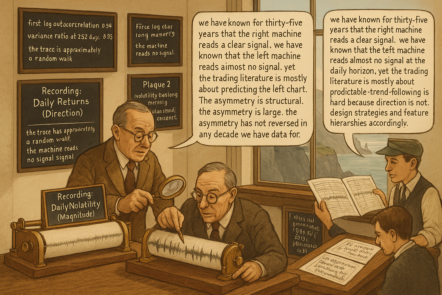
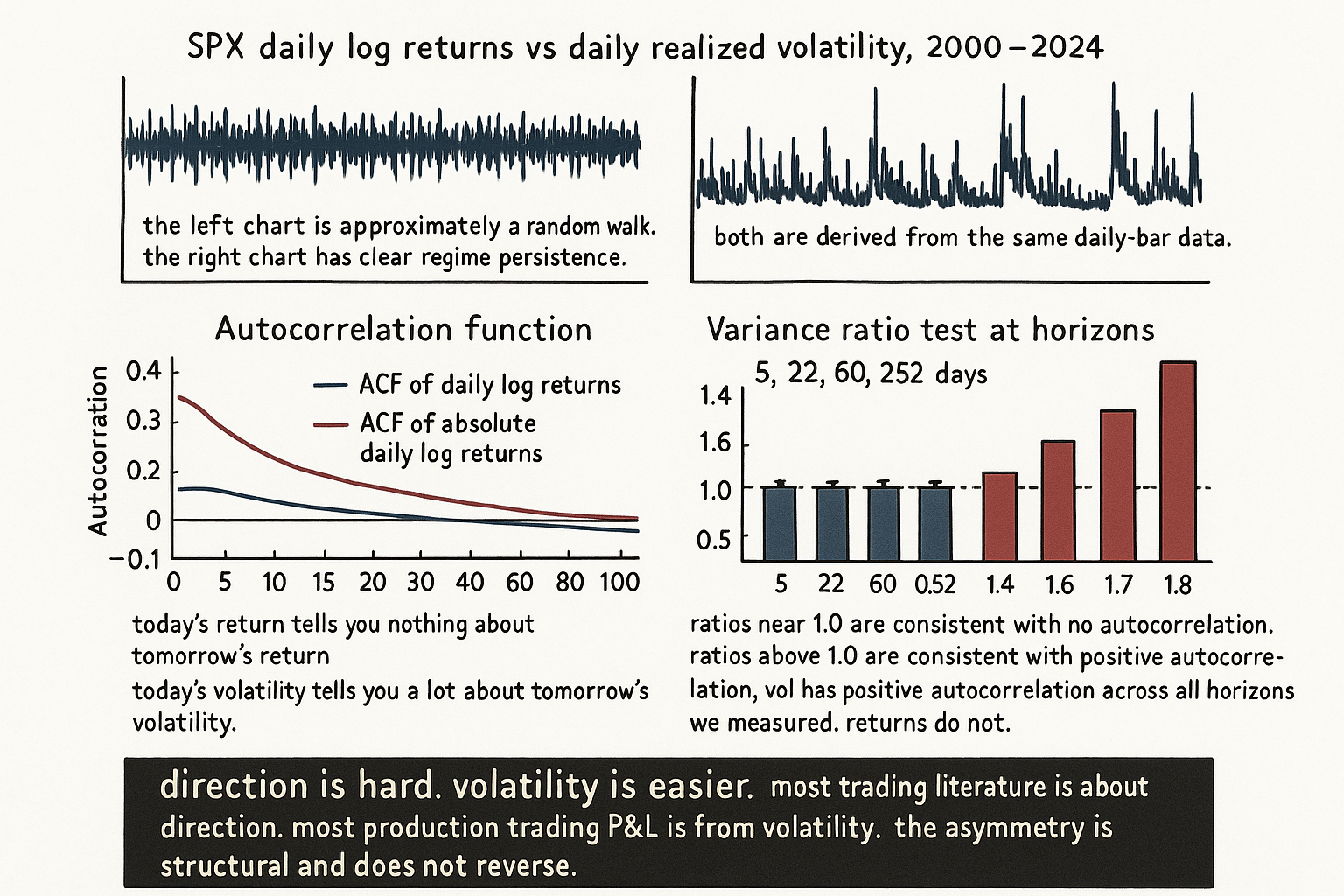
Compute the first-lag autocorrelation of daily log returns on SPX from 1990 to 2024. The value is approximately -0.04. Compute the same statistic on the absolute value of daily log returns (a proxy for daily volatility). The value is approximately +0.27. The two numbers say something structural: returns have almost no day-to-day memory, while volatility has strong day-to-day memory. Compute the variance ratio of the realized vol time series at horizons of 5, 22, 60, and 252 days. All four exceed 1.0, with the longest horizon at approximately 1.8. The same variance-ratio test on returns hovers near 1.0 at all horizons. Volatility moves are persistent. Return moves are not.
This is the core empirical fact that should govern most decisions in a trader's research workflow. Direction is hard to predict because direction is approximately a random walk on most timescales. Volatility is comparatively easy to predict because volatility has long memory. Yet most retail trading literature, technical analysis, and chart-pattern research is dedicated to predicting direction, while the structurally easier prediction (volatility) is treated as a sizing detail rather than the main signal. The article "Volatility Regimes and Strategy Survival" gave the operational gating framework. This article covers the underlying reason that the vol-regime gating decision is the highest-leverage decision in the pillar: vol drifts on a timescale that is short enough to matter for almost any strategy, while trend drifts on a timescale that is too long to easily exploit.
Measuring the persistence asymmetry
Three diagnostics, each pointing to the same conclusion.
Diagnostic 1: autocorrelation function. The first-lag autocorrelation of daily SPX returns from 1990 to 2024 is approximately -0.04. The autocorrelation decays to zero within 1 to 2 lags. The autocorrelation of absolute returns starts at +0.27, remains above +0.15 at lag 10, above +0.08 at lag 22, and only crosses zero around lag 100 (4 to 5 months). The integrated autocorrelation of vol exceeds the integrated autocorrelation of returns by a factor of 50 to 100.
$$ \text{ACF}_r(k) = \frac{\text{Cov}(r_t, r_{t-k})}{\text{Var}(r_t)}, \qquad \text{ACF}_{|r|}(k) = \frac{\text{Cov}(|r_t|, |r_{t-k}|)}{\text{Var}(|r_t|)} $$
The interpretation is direct: today's return tells you almost nothing about tomorrow's return; today's volatility tells you a lot about tomorrow's volatility.
Diagnostic 2: variance ratio test. For a stationary process with no autocorrelation, the variance of the k-period sum is k times the 1-period variance. The variance ratio is the empirical k-period variance divided by k times the 1-period variance.
$$ \text{VR}(k) = \frac{\text{Var}(X_t + X_{t-1} + \dots + X_{t-k+1})}{k \cdot \text{Var}(X_t)} $$
For SPX daily returns: VR(5) ≈ 1.02, VR(22) ≈ 1.08, VR(60) ≈ 1.04, VR(252) ≈ 0.95. All near 1.0, consistent with returns being approximately a random walk on these horizons. For SPX daily realized vol (or absolute returns): VR(5) ≈ 1.4, VR(22) ≈ 1.6, VR(60) ≈ 1.7, VR(252) ≈ 1.8. The variance ratios climb monotonically with the horizon, consistent with strong long memory.
Diagnostic 3: half-life of mean reversion. Fit an AR(1) model to each series. The half-life is the number of bars for the AR(1) shock to decay by half.
$$ \text{half-life} = -\frac{\ln 2}{\ln \rho}, \qquad \rho = \text{AR(1) coefficient} $$
For SPX daily returns: ρ ≈ -0.04, half-life is undefined (no mean reversion or anti-persistence at one lag). For SPX log realized vol: ρ ≈ 0.95, half-life ≈ 14 days. For SPX log realized vol on monthly data: ρ ≈ 0.85, half-life ≈ 4 months. Volatility shocks decay measurably within weeks to months. Return shocks decay within hours to days (and the small negative autocorrelation is more about microstructure than predictability).
Volatility has long memory
Three structural reasons.
Reason 1: information arrival is itself clustered. Volatility scales with the rate of arrival of new information that traders disagree about. Information arrival is bursty (earnings releases, macroeconomic announcements, geopolitical shocks come in clusters with quiet periods between). The vol process inherits the clustering of the information process.
Reason 2: volatility creates more volatility. A large move triggers margin calls, position liquidations, hedging flows, and forced rebalancing by passive funds. Each of these creates additional flow that is itself volatile. The mechanism is amplifying rather than damping. A 5-sigma return on day t increases the conditional probability of another large return on day t+1 because the day-t move has set off cascades that take days to unwind.
Reason 3: volatility-of-volatility is also non-stationary. The conditional volatility of the vol process itself drifts across regimes. In low-vol regimes, vol clusters tightly around its mean. In high-vol regimes, vol can swing widely from day to day. The two-level non-stationarity (drift in vol mean, drift in vol-of-vol) compounds the persistence.
Direction has no long memory
Three structural reasons that mirror the above.
Reason 1: arbitrage damps directional persistence. If returns had a +0.3 first-lag autocorrelation on a daily horizon (vol-like persistence), participants would buy after up days and sell after down days, eroding the autocorrelation until the trade is no longer profitable. The market's no-free-lunch boundary prevents directional persistence from accumulating beyond the boundary set by transaction costs.
Reason 2: directional flow is two-sided. A large up move creates buyers (trend followers) and sellers (rebalancing, profit-taking, mean-reverters). The two flows roughly cancel on the next day. A large vol move creates only one type of follow-on flow (more hedging, more margin calls), which is structurally one-sided.
Reason 3: directional opinions are diverse. At any moment, the market contains long-horizon investors, short-horizon traders, hedgers, arbitrageurs, and noise traders. Their directional views are heterogeneous. The aggregate direction at the daily horizon is a weighted average of many competing views and the residual is approximately mean-zero noise. Volatility, by contrast, is one-dimensional: everyone agrees that "the market is volatile" or "the market is calm". The agreement amplifies the persistence.
The asymmetry is not absolute. Long-horizon momentum and trend following do work, with annualized Sharpes of 0.4 to 0.7 on most asset classes across decades. The article "Equity 12-1 momentum factor decay" (covered in "Slow Wandering: The Most Dangerous Type of Market Change") frames the long-term decay of one specific directional anomaly. The point of the asymmetry is operational: directional edges exist, but they are smaller per unit of variance and harder to extract than vol-regime edges.
Operational implications
Five consequences for strategy design and portfolio operation.
Implication 1: vol-targeting works. The classical mean-variance position-sizing rule (set position size inversely to forecast volatility) is the simplest application of vol's predictability. Because the forecast vol is reasonably accurate at short horizons, the position-sized portfolio has more stable realized vol than the unscaled portfolio. The article "Why ATR Normalization Is More Than a Volatility Trick" covered the indicator-level version of this technique.
Implication 2: vol-of-vol-targeting is the next-order refinement. A portfolio that targets a fixed vol level but does not adjust for vol-of-vol underestimates risk in unstable-vol regimes. The refined rule scales position size by the inverse of forecast vol times an adjustment for forecast vol-of-vol. The refinement matters most for short-vol strategies where vol-of-vol regime detection is the difference between profitability and ruin.
Implication 3: trend-following needs more samples than vol-trading. To detect a directional edge with statistical confidence, the trader needs many independent samples because each sample carries low signal-to-noise. To detect a vol regime, the trader needs few samples because the regime is persistent. A 50-sample directional backtest is approximately worthless; a 50-sample vol-regime classification is approximately reliable.
Implication 4: leverage is asymmetric across strategy types. A vol-trading strategy with predictable vol can run at higher leverage than a directional strategy with unpredictable direction, at equal Sharpe, because the vol-trading drawdown distribution is tighter. The asymmetry is masked in standard reporting because both strategies are presented at constant vol target. The Sharpe-equivalent leverage is different.
Implication 5: backtest sample-size requirements differ. The article "Trade-Count Thresholds for Backtest Reliability" later in this pillar gives the general framework. The specific lesson here: vol-prediction backtests can validate on shorter samples than direction-prediction backtests because the underlying signal is stronger.
Indicator design implications
The article block on indicator engineering (Pillar 2) covered how to construct features. The volatility persistence has direct implications for which features carry the most information.
Volatility-derived features (ATR, GARCH-fitted vol, realized vol, range/Parkinson estimators) carry strong predictive information about future volatility. The signal is large enough to overcome estimation noise on samples of 100 to 500 observations.
Direction-derived features (momentum, trend strength, signed returns) carry weak predictive information about future direction. The signal is small enough that it requires 1000 to 10000 observations and very careful denoising. The article "Why Predictive Power Often Lives in the Tails" framed one specific case where the directional signal becomes detectable (in the extremes of the indicator distribution).
The asymmetry argues for a feature-engineering hierarchy: the strongest features are vol-derived, the moderately strong features are vol-conditional or vol-normalized direction features (e.g., the signed return divided by the contemporaneous ATR), and the weakest features are raw direction features.
Anti-patterns
Five mistakes that follow from ignoring the persistence asymmetry.
Anti-pattern 1: building a directional strategy without a vol filter. A momentum strategy without a vol-regime gating rule is on during low-vol regimes (where momentum is too small to overcome costs) and during high-vol regimes (where momentum reverses in fast and abrupt swings). Add the vol filter; the gated strategy has a higher Sharpe than the ungated version on most asset classes.
Anti-pattern 2: using a single-horizon vol estimator across all use cases. The right horizon depends on the use case. Position sizing calls for a fast estimator (5 to 10 days) to track current vol. Strategy gating calls for a slower estimator (22 to 60 days) to identify regime. Tail-risk hedging calls for the longest estimator that still tracks the regime. A single 22-day vol used everywhere underestimates the regime in transitions and overestimates short-term sizing precision.
Anti-pattern 3: assuming vol forecasts have the same error distribution as direction forecasts. Vol forecast errors are right-skewed (vol can spike but cannot go below zero) and the forecast error variance scales with the level. Direction forecast errors are approximately symmetric but with much higher variance per unit time. Position-sizing rules need to be calibrated to the right error distribution; using a Gaussian approximation for vol forecast errors underestimates the tail risk.
Anti-pattern 4: cross-asset vol comparisons without scale correction. SPX 14% annualized vol, EURUSD 8% annualized vol, and crude oil 28% annualized vol are not directly comparable because the underlying processes have different return distributions. Vol-regime classification needs to be done in each asset's own scale (rolling percentiles, z-scores against the asset's own history) rather than in absolute units.
Anti-pattern 5: assuming GARCH parameters are stationary across regimes. The GARCH persistence parameter (the AR coefficient on conditional variance) is itself non-stationary across decades. The 1990s SPX GARCH-fitted persistence is different from the 2010s. Re-fit the model on rolling windows; do not assume the model parameters are constants.
Decision matrix
| Use case | Vol estimator | Direction estimator | Notes |
|---|---|---|---|
| Position sizing | 10-day realized | None | Use inverse vol scaling; refine with vol-of-vol if available |
| Strategy gating | 22-60 day realized | None | Use thresholds with hysteresis from prior article |
| Tail-risk hedging | 60-252 day realized | None | Match hedge horizon to risk horizon |
| Trend following | 252-day realized for filter | 12-1 momentum on returns | Disable trend when vol below floor |
| Mean reversion | 22-day realized for gating | 5-day reversal on returns | Disable reversion when vol above ceiling |
| Vol-carry | All horizons (regime detect) | None | Implied-realized spread is the signal; vol-of-vol is the gate |
| Volatility prediction | GARCH(1,1) or HAR | None | Vol persistence makes this tractable; refit annually |
| Direction prediction | Vol-conditional features | Many candidates, low signal-to-noise | Combine with vol filter, accept low IR |
The matrix maps the use case to the dominant signal type. The pattern: vol estimators dominate, direction estimators are supplementary, and strategies that can be expressed as vol-prediction or vol-conditional are typically more reliable than pure direction strategies.
Visualizing the persistence asymmetry
KEY POINTS
- Direction is approximately a random walk on daily-to-monthly horizons. First-lag autocorrelation of SPX daily returns is approximately -0.04. Variance ratios at 5, 22, 60, 252 days hover near 1.0.
- Volatility has strong long memory. First-lag autocorrelation of SPX absolute daily returns is approximately +0.27. Variance ratios climb from 1.4 at 5 days to 1.8 at 252 days. The half-life of vol shocks is 2-4 weeks at daily resolution and 4 months at monthly resolution.
- Three structural reasons for vol persistence: information arrival is bursty, volatility creates volatility through forced flows (margin calls, hedging, rebalancing), vol-of-vol is itself non-stationary so the persistence compounds.
- Three structural reasons direction lacks persistence: arbitrage damps directional autocorrelation to the boundary set by transaction costs, directional flow is two-sided (buyers and sellers respond to the same move), directional opinions are heterogeneous and the aggregate residual is mean-zero.
- The asymmetry is operational. Vol-targeting works because vol forecasts are accurate enough at short horizons. Trend-following and momentum work because directional edges exist but they are smaller per unit variance than vol-regime edges and require many more samples to validate.
- Operational consequence: a 50-sample directional backtest is approximately worthless. A 50-sample vol-regime classification is approximately reliable. Sample-size requirements differ by an order of magnitude between vol-prediction and direction-prediction strategies.
- Feature engineering hierarchy: vol-derived features carry strong predictive information, vol-conditional or vol-normalized direction features (e.g., signed return / ATR) carry moderate information, raw direction features carry weak information.
- Anti-pattern: building a directional strategy without a vol filter. The same momentum signal is profitable in some vol regimes and loss-making in others; the gated version has a higher Sharpe.
- Anti-pattern: a single-horizon vol estimator across all use cases. Position sizing calls for 10 days, gating for 22-60 days, tail-risk hedging for 60-252 days. One window does not serve all.
- Anti-pattern: cross-asset vol comparisons without scale correction. SPX, EURUSD, and crude have different return distributions; vol-regime classification must be done in each asset's own scale.
- Anti-pattern: assuming GARCH or HAR persistence parameters are stationary. The persistence itself drifts across decades. Refit on rolling windows.
- The current article gives the empirical fact and structural reasons. The next article in the publication ("How to Make Indicators More Stationary") covers the toolset for transforming raw features into stationary inputs that strategies can consume reliably.
References
- Testing and Tuning Market Trading Systems - Timothy Masters (Amazon)
- Data Mining Algorithms in C++ - Timothy Masters (Amazon)
- Stylized Facts of Asset Returns and Their Implications for Quantitative Finance
- Volatility Clustering in Financial Markets: Empirical Facts and Agent-Based Models
- Financial Time Series: Stylized Facts for the Mexican Stock Exchange
- Spurious Predictability in Financial Machine Learning - arXiv
- Futuretesting Quantitative Strategies by Daniel Alexandre Bloch
- Fire sales forensics: measuring endogenous risk - NYU Stern
- Online Quantitative Trading Strategies - NYU Stern
- Improving the Robustness of Trading Strategy Backtesting with