3. Robust Systems Lab May 28, 2026 11 min

3.6 Volatility Regimes and Strategy Survival

Lifetime Sharpe is regime-weighted, not favorable-year. Each strategy has a vol regime where it lives and one where it dies. Gate at deployment, calibrate against the full distribution.

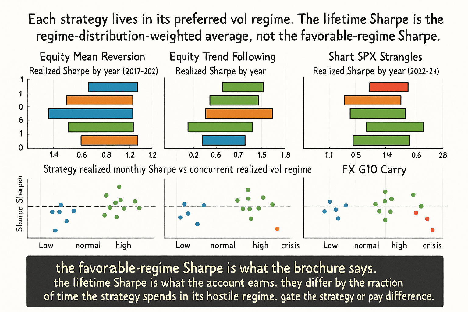
A diversified multi-strategy book runs four strategies side by side: equity mean reversion (5-day reversal on the SPX 500 universe), equity trend following (12-1 momentum on the same universe), short-volatility carry (selling SPX 30-delta strangles weekly), and FX carry (long G10 highest-yielders, short lowest-yielders). The book is sized at 10% annualized volatility target. Across calendar 2017 to 2024 the realized P&L per strategy looks very different by year, with the volatility regime each year was in explaining almost all of the difference.

In 2017 (full year, SPX realized vol approximately 7%), mean reversion delivered Sharpe 1.4, trend following Sharpe 0.2, short vol Sharpe 2.6, FX carry Sharpe 1.1. In 2018 (SPX realized vol approximately 17%, with the February vol spike and Q4 selloff), mean reversion Sharpe -0.4, trend following Sharpe 0.6, short vol Sharpe -2.8 (the year of the XIV blow-up), FX carry Sharpe 0.0. In 2019 (vol approximately 12%), mean reversion 0.8, trend following 0.7, short vol 1.6, FX carry 0.4. In 2020 (vol approximately 35%, Covid spike), mean reversion 1.2 (the rebound was a giant mean-reverting move), trend following 1.5 (sustained directional moves in many assets), short vol -3.5 (the March vol spike was a 5-sigma event for the strategy), FX carry -1.2. In 2021 (vol approximately 14%), mean reversion 0.6, trend following 0.4, short vol 1.9, FX carry 0.3. In 2022 (vol approximately 22% with persistent uptrend then drawdown), mean reversion -0.1, trend following 1.8, short vol 0.0, FX carry 1.4 (the dollar trend was strong). In 2023 (vol approximately 13%), mean reversion 0.7, trend following 0.5, short vol 1.7, FX carry 0.6. In 2024 (vol approximately 12%), mean reversion 0.6, trend following 0.4, short vol 1.5, FX carry 0.5.

The lifetime Sharpe of each strategy is set first and foremost by how the realized volatility regime distribution stacks up against the strategy's regime preference. Short vol is the most extreme example: 2017 alone delivered enough P&L to cover 2018 and 2020 combined, and the lifetime Sharpe across 2017 to 2024 is approximately 0.5, not the 2.0 that the median year suggests. The article "Why Systems Work Until They Don't" framed the four mechanisms of strategy decay; this article zooms in on the most operationally important regime axis (volatility) and shows how to gate strategies on that axis. The next article in the publication ("Why Volatility Is More Non-Stationary Than Trend") covers the empirical fact that makes volatility-regime gating the highest-leverage decision in this pillar.

Defining the volatility regime

Three regime axes, each measurable in real time.

Axis 1: realized volatility level. The 22-day or 60-day annualized standard deviation of daily returns. Three rough levels for SPX (each market has its own scale): low vol below 10% annualized, normal vol 10 to 18%, high vol above 18%. Crisis regimes (>30%) are in the long tail of the high-vol distribution.

$$ \sigma_t^{(\text{realized})} = \sqrt{252} \cdot \sqrt{\frac{1}{N-1} \sum_{i=0}^{N-1} (r_{t-i} - \bar{r}_t)^2}, \qquad N = 22 \text{ or } 60 $$

Axis 2: volatility-of-volatility. The standard deviation of the rolling realized vol estimate itself, on a longer window. High vol-of-vol regimes are unstable (vol can spike or collapse); low vol-of-vol regimes are stable. Vol-of-vol matters because it determines whether short-vol strategies will be hit by a sudden vol expansion.

Axis 3: implied versus realized vol spread. The 30-day SPX implied volatility (VIX) minus the 22-day realized vol. The spread is positive on average (insurance premium) and widens before crises and tightens during low-stress regimes. The spread is the headline P&L driver for short-vol strategies and a useful regime signal for the broader market.

A fourth axis (the volatility surface curvature, the term structure of VIX, the volatility skew) is useful at the high-frequency strategy level but optional for first-order regime classification.

Mapping strategies to regime preference

Each strategy class has a preferred vol regime where it earns its full edge and a hostile regime where it loses money structurally.

Equity mean reversion (5-day reversal, pairs trading, statistical arbitrage). Lives in low-to-normal vol regimes with weak trends. Earns from short-term overreaction and noise. In high-vol or trending regimes, the "overreaction" is real information and the strategy fades real moves until it gets stopped out. Hostile regime: high vol with directional persistence.

Equity trend following (12-1 momentum, breakout systems). Lives in normal-to-high vol regimes with directional moves. Earns from sustained directional persistence. In low-vol regimes the directional moves are too small to overcome transaction costs and stops. In choppy high-vol with no direction the strategy whipsaws. Hostile regime: low vol with no trend, or high vol with chop.

Short volatility (selling SPX strangles, VIX futures shorts, vol-carry overlays). Lives in low-to-normal vol regimes that are stable. Earns the implied-realized vol premium. In vol-expansion regimes the strategy can lose 30 to 50% in a single week or month. The 2018 February spike, the 2020 March spike, and the multiple smaller spikes in 2022 to 2024 are the canonical hostile events. The article "Why Profit Factor Can Lie" later in this pillar covers the issue that short-vol headline statistics often hide.

FX carry (long high-yielders, short low-yielders). Lives in low-to-normal vol regimes with stable risk appetite. Earns interest-rate differential. In high-vol regimes the carry currencies (high-yielders are typically EM or commodity-linked) sell off violently. The carry P&L tends to "go up the stairs and down the elevator" because vol regimes flip from low to high quickly.

Cross-sectional equity factors (value, quality, low-vol, momentum). Each factor has its own vol-regime preference. Quality and low-vol perform best in high-vol regimes (defensive bid). Value performs best in transitions. Momentum performs worst at vol-regime turning points (the "momentum crashes" of 2009 and 2020 are the canonical examples).

The mapping is empirical, calibrated from history rather than derived from first principles. The point of having an explicit mapping is operational: when the live volatility regime moves out of the strategy's preferred regime, the strategy's allocation should be reduced or zeroed.

Real-time regime classification

Three classifiers, with increasing sophistication.

Classifier 1: deterministic threshold. Compute the 22-day realized vol. Map to a regime label by fixed thresholds (e.g., low if below the 33rd percentile of the long-run distribution, normal between 33rd and 67th, high above 67th). Cheap, transparent, reasonable for first-pass gating. Weakness: sharp transitions between regimes can produce frequent flips at the threshold.

Classifier 2: smoothed threshold with hysteresis. Same as classifier 1 but with two thresholds per boundary (a higher threshold to enter "high vol" and a lower threshold to exit). The hysteresis prevents flip-flopping at the boundary. The thresholds are calibrated against the historical regime distribution.

Classifier 3: regime-switching model. Fit a Markov-switching model to the realized vol time series. The model produces a posterior probability of being in each regime at each time. Use the posterior probability as a continuous gating signal rather than a binary classifier. The article "How to Make Indicators More Stationary" later in this pillar covers the broader use of regime-switching machinery.

The choice depends on the strategy. Short-vol strategies benefit from the fastest classifier with the lowest false-positive rate (a missed regime shift is a 30 to 50% loss). Mean-reversion and trend-following strategies tolerate a slower classifier with hysteresis (a false positive costs the strategy a few weeks of edge; a missed regime shift costs roughly 20 to 30 basis points of underperformance per month).

Operational gating rules

Five rules that the diversified-book example above suggests.

Rule 1: short-vol strategies disable when the implied-realized vol spread compresses below a threshold. The compression is the warning that the insurance premium is no longer adequate compensation for the tail risk. A compressed spread plus a vol-of-vol uptick is the signature of an imminent vol expansion.

Rule 2: trend-following strategies disable in low-vol regimes below a threshold. The directional moves are too small to overcome transaction costs and stops. Re-enable when the realized vol crosses back above the threshold sustainedly (with hysteresis).

Rule 3: mean-reversion strategies disable in high-vol regimes above a threshold. The "overreaction" in high vol is real information and the reversion thesis fails. Re-enable when realized vol drops below the threshold sustainedly.

Rule 4: FX carry strategies disable when global cross-asset vol exceeds a threshold (VIX above 25 or equivalent). The carry-currency drawdown in high-vol regimes is structural and large. Re-enable when global vol normalizes.

Rule 5: at the portfolio level, do not let any one strategy carry more than 30% of the active risk budget when the regime favors it. The regime-favorable sizing is tempting (the in-favor strategy earns the most P&L per unit risk in its regime) but creates portfolio-level fragility when the regime turns. Maintain regime-diversified weights even when one regime is the current state.

The vol regime distribution and its asymmetry

The realized-vol distribution is right-skewed. Most days are low or normal vol; the tail is in the high-vol regime. Across SPX 1990 to 2024, approximately 40% of days are low vol (below 10% annualized), 45% are normal (10 to 18%), 12% are high (18 to 30%), 3% are crisis (above 30%). The fraction of total return variance contributed by the high-vol and crisis days is much larger than the fraction of days, because variance scales with squared returns.

$$ \frac{\sum_{t \in \text{high vol}} r_t^2}{\sum_{t \in \text{all days}} r_t^2} \approx 50\% \text{ from } 15\% \text{ of days} $$

The asymmetry has two operational implications. First, a strategy that is on during high-vol days and off during low-vol days is exposed to most of the year's risk in a small number of days. Second, the in-sample vs out-of-sample regime mismatch (covered in "Why OOS Failure Is Often a Stationarity Failure") matters most when the IS and OOS differ in their high-vol-day count, because most of the variance is concentrated in those days.

Anti-patterns

Five mistakes specific to volatility-regime management.

Anti-pattern 1: assuming the realized vol distribution is stationary. The unconditional vol distribution drifts across decades (1990s averaged 14% SPX vol, 2000 to 2008 averaged 18%, 2010 to 2019 averaged 14%, post-2020 has averaged 18%). Threshold rules calibrated on one decade may be wrong on another. The article "Why Volatility Is More Non-Stationary Than Trend" covers this drift in detail.

Anti-pattern 2: using a single vol threshold across all strategies. Each strategy has a different regime preference and a different threshold. A unified "high vol = risk off" rule reduces the diversified-book Sharpe by averaging across regime-mismatched strategies. Each strategy needs its own gating rule.

Anti-pattern 3: short vol presented as a high-Sharpe strategy without the tail. The headline Sharpe of short vol across normal-vol years is 1.5 to 2.5. The lifetime Sharpe across the full vol-distribution including the tails is 0.3 to 0.7. The headline number is correct conditional on the regime; the lifetime number is correct unconditionally. Strategy evaluation needs the unconditional number.

Anti-pattern 4: vol gating as a substitute for sizing. A strategy that is on in its favorable regime and off in its hostile regime still needs to be sized at the portfolio level. The favorable regime can produce 5-sigma-of-the-strategy moves that swamp the portfolio if the position is too large. Gating reduces the worst-regime exposure but does not eliminate it.

Anti-pattern 5: backtesting a strategy that is implicitly gated by survivor bias. The strategy "happened to be off" during the 2018 vol spike or the 2020 March spike because the parameters were tuned on a window that excluded those events. The backtest reports a strong Sharpe; the live deployment will be on during the next equivalent event. Verify the gating rule is causal (uses only past data) and that the backtest applies the same gating across the entire history including hostile regimes.

Decision matrix

Strategy class	Preferred regime	Hostile regime	Gating rule
Equity 5-day reversal	Low-to-normal vol, weak trend	High vol with persistent direction	Disable when realized vol > 22%
Equity 12-1 momentum	Normal-to-high vol with direction	Very low vol or whipsaw high vol	Disable when realized vol < 8%
Short SPX strangles	Low-to-normal vol, low vol-of-vol	Vol expansion	Disable when (implied - realized) < 1% or vol-of-vol > 80th pct
FX G10 carry	Low global vol, stable risk	High global vol, risk-off	Disable when VIX > 25
Cross-sectional value	Transition regimes	Persistent low-vol bull	Continuous, soft gating
Cross-sectional momentum	Trending regimes	Vol-regime turning points	Reduce at vol-regime transitions
Quality / low-vol factor	High vol (defensive bid)	Low vol (chasing trash)	Continuous, soft gating
Trend-following CTA on multi-asset	Multi-asset regime divergence	Sustained low-vol risk-on	Continuous, with vol filter on each asset

The matrix is operational, illustrative thresholds. Each portfolio needs its own calibration against its own historical sample and risk budget.

Visualizing strategy survival across vol regimes

KEY POINTS

Strategy lifetime P&L is set first and foremost by the volatility regime distribution the strategy sees during deployment. The favorable-regime Sharpe is the brochure number; the lifetime Sharpe is the regime-distribution-weighted average and is typically much lower.
Three regime axes are measurable in real time: realized volatility level (22- or 60-day annualized std), vol-of-vol (rolling std of the realized vol estimate), implied-minus-realized spread (VIX minus 22-day realized).
Mapping strategies to regime preference: equity mean reversion lives in low-to-normal vol with weak trend; equity trend following lives in normal-to-high vol with direction; short volatility lives in low-to-normal vol with low vol-of-vol; FX carry lives in low global vol with stable risk appetite.
Each strategy has a hostile regime where it loses money structurally. Mean reversion in high vol with persistent direction. Trend following in low vol or whipsaw high vol. Short vol in vol-expansion events. FX carry in cross-asset vol spikes.
Real-time regime classification: deterministic thresholds with hysteresis are sufficient for slow-moving strategies; Markov-switching posterior probabilities are appropriate for fast-moving short-vol strategies where missed regime shifts produce 30 to 50% losses.
Five operational gating rules: disable short vol when the implied-realized spread compresses, disable trend-following in very low vol, disable mean reversion in high vol with persistent direction, disable FX carry when global VIX exceeds 25, cap any single strategy at 30% of active risk budget regardless of current regime favorability.
The realized-vol distribution is right-skewed. Across SPX 1990 to 2024, low-vol days are 40% of the sample, normal 45%, high 12%, crisis 3%. The high-vol and crisis days contain approximately 50% of the squared-return variance. Strategy exposure during these days drives most of the lifetime P&L variance.
Anti-pattern: assuming the unconditional vol distribution is stationary. Vol-distribution drift across decades shifts threshold-rule calibration. The next article in the publication ("Why Volatility Is More Non-Stationary Than Trend") covers this in detail.
Anti-pattern: short-vol headline Sharpe (1.5 to 2.5 in favorable years) presented as the unconditional Sharpe (0.3 to 0.7 across full distribution including tails). Strategy evaluation needs the unconditional number.
Anti-pattern: vol gating as a substitute for sizing. Gating reduces hostile-regime exposure but does not eliminate it. Position sizing must still cap the portfolio impact of a single strategy's worst-regime loss.
The current article gives the operational regime-gating framework. The article "Why Volatility Is More Non-Stationary Than Trend" covers the empirical fact that makes vol gating the highest-leverage decision in this pillar.