3. Robust Systems Lab May 28, 2026 13 min

3.3 Why Systems Work Until They Don't

Every strategy has a finite life. Four decay mechanisms: crowding, regime drift, microstructure, capacity. Size against half-life. Run a shadow book. Write the decommission policy at deployment.

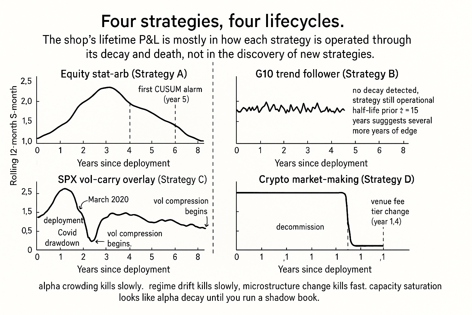
A trading shop runs four strategies in production. Strategy A is an equity-pairs mean-reverter built in 2014 on a basket of 200 large-cap US names. Strategy B is a CTA-style trend follower on the G10 FX block built in 2017. Strategy C is a vol-carry overlay on SPX index options built in 2019. Strategy D is an intraday market-making book on a single Tier-1 crypto venue built in 2022. As of 2025, the four strategies have produced very different lifetime trajectories.

Strategy A peaked in 2016 to 2018 (Sharpe 1.4) and decayed through 2019 to 2024 (Sharpe 0.6 by 2023, near-zero in 2024). The shop pulled it in late 2024 after CUSUM on the realized predictive R-squared crossed the decommission threshold. Strategy B has been stable: the realized Sharpe across 2017 to 2025 is 0.7 with no clear trend. The trend-following premium on G10 has not crowded out at the multi-week horizon at which the strategy operates. Strategy C ran beautifully through 2019 to early 2020 (Sharpe 1.8), produced a 22% drawdown in March 2020, recovered, and has run a deteriorating Sharpe (1.0, 0.5, 0.2) through 2022 to 2024 as the SPX implied-vs-realized spread compressed. The shop is keeping it on at a halved allocation while research finishes a vol-skew variant. Strategy D ran for fourteen months at Sharpe 2.4 and then died abruptly when the venue's order-book microstructure changed (a fee-tier overhaul that doubled the effective spread on the strategy's order sizes). The shop pulled it within two weeks. The replacement is in research and may or may not work.

Four strategies, four lifecycles. Each was right when it was built, each delivered some edge, each will eventually be replaced. The shop's lifetime P&L depends less on which strategies it found and more on how it managed the inevitable decay of each one. The prior articles in the publication ("Stationarity: The Word Every Trader Ignores Until It Kills the Strategy" and "Slow Wandering: The Most Dangerous Type of Market Change") gave the diagnostic machinery for detecting when the substrate is changing. This article generalizes the diagnostic problem to the steady-state portfolio question: how to operate a portfolio of strategies that all eventually die, how to size each one against its expected remaining life, and how to budget research bandwidth around the replacement problem rather than the discovery problem.

The lifecycle of a trading strategy

Four stages, distinguishable by the relationship between realized and expected performance.

Stage 1: discovery and validation. The strategy is built, backtested, walk-forward validated, and stress-tested. The realized OOS performance roughly matches the in-sample backtest after honest cost assumptions. The strategy passes the Pillar 3 testing checklist (covered across the rest of this pillar). Duration: typically 3 to 12 months of research.

Stage 2: live deployment. The strategy is funded and runs at full target allocation. Realized performance tracks the backtested expectation within the expected statistical band. The trader monitors stationarity diagnostics on the input features, drift detectors on the prediction quality, and standard P&L metrics. Duration: typically 1 to 5 years for a healthy strategy.

Stage 3: decay. Realized performance starts deteriorating relative to the deployment-era baseline. The deterioration may be a slow drift (covered in detail in "Slow Wandering: The Most Dangerous Type of Market Change") or a sequence of small abrupt shifts (regime breaks, microstructure changes). Drift detectors trigger one or more alarms. The trader takes one of three actions: continue at reduced allocation, retrain on recent data, or begin decommission. Duration: typically 6 months to 2 years.

Stage 4: death. The strategy is decommissioned. The decommission may be triggered by a hard alarm (drawdown exceeding policy, OOS Sharpe below threshold for N months, structural change in the substrate that invalidates the model). It may also be a research-driven retirement (a better strategy supersedes the old one). The capital is reallocated to other strategies or held in cash pending the next deployment. Duration: instantaneous (the decommission decision) followed by post-mortem.

Four mechanisms of decay

Each mechanism has a different timescale and a different defense. Diagnosing which mechanism is killing a specific strategy is the hard part.

Mechanism 1: alpha crowding. Other participants discover the same edge and trade it, eroding the realized return. Crowding shows up as a slow Sharpe decline, often accompanied by widening transaction costs (slippage on entry and exit grows as more capital chases the same trades). The 12-1 equity momentum factor decay covered in "Slow Wandering: The Most Dangerous Type of Market Change" is the canonical example. Defense: the strategy capacity is finite and known approximately. Size below capacity. Reduce allocation as crowding increases.

Mechanism 2: regime drift in the substrate. The market's structural parameters change. The prior article block covered this in detail. Examples: G10 yield convergence killing FX carry, SPX implied-vs-realized vol compression killing vol-selling overlays, equity-bond correlation flips invalidating risk-parity priors. Defense: monitor the substrate-level features that the strategy depends on. Disable when the features move outside the deployment regime.

Mechanism 3: microstructure change. The exchange, market-maker, or fee structure changes. The change may be an obvious one (a fee tier overhaul, a tick-size change, the introduction of a new auction format) or a subtle one (a large new participant changes the order-flow composition). Microstructure-dependent strategies (market-making, latency arbitrage, order-flow prediction) are most exposed. Defense: maintain a venue-level changelog, monitor execution quality metrics (effective spread, fill rate, markout) at high frequency, decommission immediately when execution quality breaks.

Mechanism 4: capacity saturation from the strategy's own growth. The shop's own capital deployed against the strategy outgrows the available liquidity. Slippage rises, fill rates drop, the realized P&L falls below the small-size backtest. This is the failure mode that scaling shops misdiagnose as alpha decay when the cause is internal. Defense: track scaled vs unscaled performance, run a small "shadow book" at a fixed reference size, compare the live large-book performance to the shadow. A divergence between the two is capacity saturation, not alpha decay.

The four mechanisms are not mutually exclusive. A strategy can be hit by crowding and capacity at the same time, or by regime drift while crowding is also accumulating. Diagnosis matters because the defense for each is different. Allocation cuts handle capacity saturation but not alpha decay. Substrate monitoring handles regime drift but not crowding. The article "How to Detect When a Trading System Is Dying" gives the operational checklist that distinguishes the mechanisms.

Modeling expected life

A simple but useful model. Treat the realized Sharpe of the strategy as a slowly decaying function of time since deployment, with stochastic noise on top.

$$ \text{SR}(t) = \text{SR}_0 \cdot e^{-t / \tau} + \eta_t, \qquad \eta_t \sim \mathcal{N}(0, \sigma_{\text{SR}}^2) $$

The half-life of the edge is τ · log 2. A strategy with τ = 5 years and SR_0 = 1.0 has an expected Sharpe of 0.74 after 2 years, 0.55 after 4 years, 0.37 after 6 years. The half-life parameter τ is a Bayesian prior, set by judgment from the population of similar strategies. A single strategy's history does not support estimating it. Reasonable priors by strategy class:

$$ \begin{array}{l|c|c} \text{Strategy class} & \tau \text{ (years)} & \text{Notes} \\ \hline \text{Equity statistical arbitrage} & 2-3 & \text{High crowding pressure} \\ \text{Cross-sectional equity factors} & 5-10 & \text{Slow decay, well-documented} \\ \text{CTA / trend following} & 10-20 & \text{Robust but capacity-limited} \\ \text{Vol-selling / carry} & 3-5 & \text{Episodic blowups} \\ \text{Market-making / microstructure} & 0.5-2 & \text{Venue-dependent} \\ \text{Macro / discretionary-systematic hybrid} & 5-10 & \text{Wide variance} \\ \end{array} $$

The values are stylized priors, not measured constants. Each strategy class has a wide distribution of realized lives and the τ above is a rough mode. The point of the prior is not precision; the point is to size positions and budget research bandwidth around a finite-life assumption rather than the implicit assumption that the strategy will work forever.

Capital allocation under finite life

A strategy's expected future P&L depends on three things: the current Sharpe, the half-life, and the funded capital. The classical Kelly fraction maximizes log-wealth assuming a stationary edge. Under finite life, the right allocation is smaller because the future expected edge is a decaying function of time.

$$ f^* = \frac{\text{SR}}{\sigma_{\text{ret}}} \cdot \frac{1}{1 + (T_{\text{horizon}} / 2\tau)} $$

The first factor is the standard mean-variance allocation. The second factor is the finite-life discount: a strategy with shorter half-life or longer planning horizon gets a smaller allocation because the expected forward edge is smaller than the current edge suggests. A strategy with τ = 2 years and a 1-year planning horizon takes a 0.8x discount. A strategy with τ = 1 year and a 5-year horizon takes a 0.29x discount; the strategy is mostly going to be dead by the time the horizon arrives.

This is the operational reason that micro-timescale strategies (market-making, latency arb) get smaller portfolio allocations than macro-timescale strategies (trend, value) at equal current Sharpe. The micro-timescale strategy is expected to die faster and the portfolio should not over-commit to a high-Sharpe strategy with short remaining life. The article "How to Evaluate a Strategy Beyond Net Profit" later in this pillar covers the broader framework for strategy evaluation under uncertainty.

The exact functional form above is a stylized model, not a derivation from first principles; the operational lesson is the direction of the adjustment, not the formula.

Portfolio-level discipline

Five rules that fall out of the finite-life assumption.

Rule 1: no single strategy carries more than 30% of the portfolio risk budget. A strategy can die in a quarter (microstructure change, regime break, sudden crowding event). The portfolio must survive any single death. The article "Why More Parameters Make a Strategy Easier to Sell and Easier to Break" gives the related point about within-strategy risk concentration.

Rule 2: the portfolio runs a research pipeline of at least 2x the production strategies. If 4 strategies are funded, at least 8 are in some stage of research, validation, or paper-trading. The pipeline is the supply curve for replacement. A shop with no pipeline has nothing to redeploy capital into when a production strategy dies.

Rule 3: every strategy has a written decommission policy at deployment time, not at decommission time. The policy specifies the metrics, thresholds, and decision rules. Examples: "decommission if 18-month rolling Sharpe falls below 0.3", "decommission if effective spread on average trade exceeds 1.5x the deployment baseline", "decommission if CUSUM on predicted-vs-realized return crosses h=5". The policy is automatic. Discretionary holds on dying strategies are the failure mode the policy exists to prevent.

Rule 4: the post-mortem is mandatory. Every decommissioned strategy gets a written analysis of which decay mechanism killed it, when the first detection signal triggered, why the trader did or did not act on it, and what the research pipeline learned. The post-mortem is the input to better priors on τ for the next strategy in the same class.

Rule 5: budget research bandwidth around replacement, not discovery. The new shop spends 100% of research time on discovering new edges. The mature shop spends 30% on discovery and 70% on monitoring, debugging, retraining, and decommissioning the existing portfolio. The mature ratio assumes the portfolio is generating most of the lifetime P&L from already-discovered strategies that are being kept alive longer through better operations.

Behavioral pitfalls

Three failure modes that show up around strategy death.

Pitfall 1: hold-and-hope on a familiar strategy. The trader has been running the strategy for years. The strategy made the trader's career. The recent underperformance "must be" a temporary drawdown. The CUSUM alarm "must be" a false positive. Personal attachment overrides the decommission policy. The cure is a written, hard-coded decommission policy that the trader cannot override without external sign-off.

Pitfall 2: premature decommission of a healthy strategy. The opposite mistake. A normal drawdown gets misclassified as the start of decay. The strategy is pulled. The drawdown was statistical noise. The trader has destroyed an asset by acting on weak evidence. The cure is discipline on the false-alarm rate of the detector. CUSUM with h=5 has a calibrated false-alarm rate (approximately one false alarm per 200 days under stationarity). Tighter thresholds than the calibration require corresponding research evidence that the trade-off is worth it.

Pitfall 3: chasing the dead strategy with retrains. The strategy underperforms. The trader retrains on the most recent year. The retrained strategy validates beautifully on 2010 to 2024 and performs poorly on 2025. The trader retrains again. The retrained strategy validates on 2010 to 2025 and performs poorly on 2026. Each retrain is fitting the recent regime that has already moved on. The cure is to recognize that retraining is a fix for slow drift and not for structural break. When the substrate has structurally changed (new microstructure regime, new macro regime, new participant mix), the retrain produces a strategy that is well-fit to a regime that no longer exists. Decommission is the right action.

Decision matrix

Decay signal	Most likely mechanism	Action
Sharpe slow decline, transaction costs rising	Alpha crowding	Reduce allocation, monitor capacity
Sharpe slow decline, transaction costs flat	Slow regime drift	Continuous walk-forward retrain
Sharpe step-down at venue change	Microstructure change	Decommission immediately, research replacement
Sharpe step-down at macro break	Regime break	Disable until regime stabilizes
Sharpe decline correlated with allocation increase	Capacity saturation	Reduce allocation, run shadow book
OOS Sharpe diverges from IS Sharpe at deployment	Backtest overfit	Decommission, post-mortem the research process
Drawdown larger than historical max but within Monte Carlo band	Statistical noise	Hold, increase monitoring
Drawdown larger than Monte Carlo 99th percentile	Real failure	Decommission per policy

The matrix is operational, not exhaustive. The article "How to Detect When a Trading System Is Dying" gives the diagnostic checklist that distinguishes the rows.

Anti-patterns

Five mistakes that show up around strategy lifecycle management.

Anti-pattern 1: assuming the discovery moment is the most important moment. The discovery is one moment in a multi-year strategy life. The harder problem is keeping the strategy operational through its decay phase and decommissioning it cleanly when the time comes. Shops that frame their job as "finding alpha" lose to shops that frame their job as "operating a portfolio of dying alphas plus a research pipeline of new ones".

Anti-pattern 2: backtesting forever to find the strategy that "doesn't decay". No strategy escapes the four decay mechanisms. The search for an immortal strategy is a search for a unicorn and the time spent searching is time not spent on operating mortal strategies well. The right framing is the actuarial one: every strategy has a finite life, the portfolio is a population of strategies in different lifecycle stages, the operator's job is the steady-state management problem.

Anti-pattern 3: no shadow book. Without a small-size shadow book running the same strategy as the funded large-size book, the operator cannot distinguish capacity saturation from alpha decay. The two failure modes look identical at the funded book's P&L level. The shadow book is cheap (a fraction of a percent of funded capital) and decisive.

Anti-pattern 4: research bandwidth dedicated to one moonshot. A research team that spends a year on one ambitious strategy has a 1-in-N hit rate where N is large. The portfolio benefits more from a research process that produces multiple modest strategies (each with τ of 3 to 5 years and Sharpe of 0.5 to 1.0) than from one ambitious strategy that may or may not survive validation. Diversification at the strategy-discovery level matters as much as diversification at the strategy-portfolio level.

Anti-pattern 5: ignoring the post-mortem. The decommissioned strategy is the most informative dataset the shop has about the decay process for that strategy class. Skipping the post-mortem skips the chance to update τ priors, refine the decommission policy, and identify research-process failures. The post-mortem is the feedback loop that makes the next strategy live longer.

Visualizing strategy lifecycles

KEY POINTS

Every trading strategy has a finite life. The question is not whether it dies but when, by which mechanism, and how the portfolio is structured to survive each death without catastrophic drawdown.
Four decay mechanisms: alpha crowding (slow Sharpe decline with rising transaction costs), regime drift in the substrate (slow Sharpe decline with stable costs), microstructure change (sharp Sharpe step-down at a venue or fee event), capacity saturation from the shop's own growth (Sharpe declines correlated with allocation increases).
Each mechanism has a different defense. Allocation cuts handle capacity. Substrate monitoring handles regime drift. Continuous walk-forward retrain handles slow drift. Immediate decommission and venue-changelog monitoring handle microstructure.
The lifecycle has four stages: discovery and validation (3 to 12 months), live deployment (1 to 5 years for healthy strategies), decay (6 months to 2 years), death (instantaneous decommission plus mandatory post-mortem).
A simple exponential-decay prior on Sharpe with strategy-class-specific half-life tau gives the right framing for capital allocation. Stylized priors: equity stat-arb tau approximately 2 to 3 years, cross-sectional equity factors tau approximately 5 to 10 years, CTA trend following tau approximately 10 to 20 years, market-making tau approximately 0.5 to 2 years.
Capital allocation under finite life is the standard mean-variance allocation discounted by a factor that depends on the ratio of planning horizon to half-life. Short-half-life strategies get smaller allocations at equal current Sharpe.
Five portfolio rules: no single strategy more than 30% of risk budget, research pipeline at least 2x the production strategies, written decommission policy at deployment time not at decommission time, mandatory post-mortem on every decommission, research bandwidth budget weighted approximately 30% discovery and 70% operations once the portfolio is mature.
Three behavioral pitfalls: hold-and-hope on a familiar strategy past its decommission criteria, premature decommission of a healthy strategy on weak evidence, chasing a dead strategy with successive retrains that fit a regime that has already moved on.
The shadow book is the cheapest tool for distinguishing capacity saturation from alpha decay. Run a small fixed-size shadow alongside the funded book and compare. A divergence is capacity. A common decline is alpha or regime.
Discovery is one moment in a multi-year strategy life. The mature shop's lifetime P&L is mostly produced by operating mortal strategies well, not by discovering immortal ones. Frame the operator's job as steady-state portfolio management, not as ongoing discovery.
The next article in the publication ("How to Detect When a Trading System Is Dying") gives the operational diagnostic checklist that distinguishes the four decay mechanisms in real time. The current article is the strategic frame; the next article is the procedural manual.