3. Robust Systems Lab May 28, 2026 10 min

3.18 The 10% Rule of Degrees of Freedom

The 10% rule: parameters / effective trades stays below 10%. Below 5% preferred. Above 10% is exploratory. Bias-to-noise scales with sqrt(p N). Count all categories.

A breakout strategy on E-mini SPX futures runs from 2010 to 2024. The backtest produces 87 trades. The strategy specification has 11 parameters by the conservative count from the article "Degrees of Freedom in Trading Systems": 4 numeric parameters (entry lookback, exit lookback, ATR period, vol-target level), 2 structural choices (breakout type, exit-rule type), 2 filter choices (volatility-regime filter, time-of-day filter), 2 sizing choices (sizing scheme, position-cap policy), 1 cost-assumption choice. The IS Sharpe is 1.4. The strategy ships in 2025.

The 10% rule applied to this strategy: parameter count divided by trade count equals 11/87 = 12.6%. The rule says the ratio should be at most 10%, with discomfort starting at 5%. The strategy at 12.6% is in the "do not deploy" zone. The team deployed anyway. The OOS Sharpe through year 1 is approximately 0.1. The post-mortem reveals that approximately 0.5 of the 1.3-Sharpe IS-OOS gap was directly attributable to the small number of trades relative to the parameter count. The other 0.8 was the structural decay of the strategy (the article "Why Systems Work Until They Don't" framed the four mechanisms). The DoF-to-trade ratio was the single largest avoidable cause of the deployment failure.

The 10% rule is a heuristic, not a theorem. The number is calibrated against thousands of backtest-to-live deployments observed across decades and across strategy families. The rule's structural justification: the trade count is the effective sample size for estimating the per-trade expectancy and Sharpe, while the parameter count is the search width over which the IS-optimal point was selected. When the search width approaches the sample size, the IS estimate is dominated by maximum-of-noise contributions and does not generalize. The 10% number is the empirical threshold below which the bias correction is small relative to the Sharpe being measured, and above which the bias correction dominates. This article gives the operational protocol for the rule.

The rule, stated formally

For a strategy with parameter count p and trade count N, the rule asserts:

$$ \frac{p}{N} \leq 0.10 \quad \Rightarrow \quad \text{deploy candidate (subject to other checks)} $$$$ \frac{p}{N} > 0.10 \quad \Rightarrow \quad \text{do not deploy. either reduce } p \text{ or extend } N \text{ or accept the strategy is exploratory} $$

The 10% threshold is an upper bound, not a target. A ratio of 1-3% is preferred. A ratio of 5-7% is workable for high-Sharpe structural strategies. A ratio of 8-10% requires the bias correction from "Degrees of Freedom in Trading Systems" to be reported alongside the raw Sharpe. A ratio above 10% is in the "exploratory only" zone.

The structural justification. The standard error of an IS Sharpe estimate with N trades is approximately 1/sqrt(N - 1). The bias from optimization across p parameters scales with sqrt(p) (each parameter is approximately one degree of freedom in the maximum-of-noise calculation). The bias-to-noise ratio is therefore approximately sqrt(p) / (1/sqrt(N)) = sqrt(p * N). For the bias to be small relative to the Sharpe, we need p / N to be small. The 10% threshold corresponds to a bias-to-noise ratio of approximately 1, which is the largest tolerable contamination of the IS estimate.

Counting p correctly

The article "Degrees of Freedom in Trading Systems" gave the eight categories. The 10% rule uses the same count. Five practical clarifications.

Clarification 1: numeric parameters are counted as the cardinality of the grid considered, not 1. An entry lookback chosen from 8 candidate values contributes 8 to the count, not 1. Anyone who counts only the chosen value is undercounting by an order of magnitude.

Clarification 2: structural alternatives count as the number of candidates considered. Choosing breakout-type from {Donchian, ATR-buffered, intraday, close-above-N-high} contributes 4 to the count.

Clarification 3: filters that were tried and removed still count. If the team considered a 200-day MA filter and decided not to include it, the choice "filter or no filter" is still a 2-way decision, and the parameter range of the filter when it was tested is also a contribution. Hidden DoF is the largest underestimation source.

Clarification 4: market and time-period selection count. The choice of "SPX rather than NDX" is a DoF if the team considered both. The choice of "2010-2024 rather than 2000-2014" is a DoF.

Clarification 5: abandoned strategies count multiplicatively. If the team tried 8 strategies and reports the best, the implicit p is multiplied by 8 because the report is the maximum across the 8 attempts.

The honest count. Apply the eight-category framework, multiply, get k_eff. For the 10% rule, the effective p is approximately log2(k_eff) (the number of bits of information the search width corresponds to). For k_eff = 1024, p_effective approximately 10. For k_eff = 1 million, p_effective approximately 20. Use p_effective in the ratio.

Counting N correctly

The trade count is the number of independent realizations of the strategy's per-trade P&L. Three subtleties.

Subtlety 1: hold time and overlap. If the strategy holds positions for 30 days and rebalances daily, the daily observations are not independent trades; the effective number of trades is approximately the total holding-period count divided by the hold time. A strategy with 5000 daily observations and 30-day holds has effective N approximately 5000 / 30 = 167 trades.

Subtlety 2: cross-sectional positions. A long-short equity strategy with 100 longs and 100 shorts rebalanced monthly over 24 months has 200 positions per month times 24 months = 4800 position-observations, but the effective number of independent decisions is closer to 24 (the number of monthly rebalances) because the longs and shorts are mostly correlated through the market and sector factor structure. Effective N is the number of independent rebalance decisions, not the position count.

Subtlety 3: regime-conditional trades. If the strategy is gated to a specific volatility regime that occurs in 30% of the sample, and the total observation count is 1000 days, the effective N is the trade count within the regime, which may be 30 or 50 trades. Strategies that are gated to rare regimes have small effective N regardless of the total observation count, and the 10% rule penalizes accordingly.

The honest count. Use the effective number of independent trade outcomes, not the total observation count, not the total position count, not the total signal count. For most strategies, effective N is between 50 and 5000.

Extending N vs reducing p

Three scenarios.

Scenario 1: the ratio is 12% with N = 100 trades and p = 12. The strategy hits a small-trade-count limit. Extending N requires longer backtests (decades, not years) or more markets (cross-asset families per "Market Personality: Why Gold, FX, Crypto, and Equities Need Different Systems"). Reducing p requires removing parameters that do not improve survival per "Why More Parameters Make a Strategy Easier to Sell and Easier to Break". For most strategies in this scenario, reducing p is faster and easier than extending N.

Scenario 2: the ratio is 12% with N = 5000 trades and p = 600. The parameter count exceeds the threshold by a wide margin. Reduce p by removing parameters that do not have a structural justification. This is the most common scenario in machine-learning-heavy strategies and ensemble systems.

Scenario 3: the ratio is 12% with N = 30 trades and p = 4. Both numbers are too small. The strategy is exploratory; the trade count is too small for any reliable estimate even at the structural-prior parameters. Extend N (apply to more markets, longer history) or accept the exploratory status and do not deploy capital at scale.

The general rule. Reducing p is usually faster, cheaper, and more effective than extending N. The article "Why More Parameters Make a Strategy Easier to Sell and Easier to Break" framed the parameter-removal discipline; the 10% rule provides the quantitative threshold for when to apply it.

Limits of the rule

Three common misinterpretations.

Misinterpretation 1: "if the ratio is below 10%, the strategy is good". The 10% rule is necessary, not sufficient. A strategy at 5% ratio with no structural premise, no economic mechanism, and no regime coverage is still bad. The rule eliminates one failure mode (parameter overfitting); it does not certify the others.

Misinterpretation 2: "if the ratio is above 10%, the strategy is bad". A strategy at 15% ratio with strong economic mechanism and clear cross-market validation may still be deployable, but with a smaller capital commitment, longer probation period, and earlier kill-switches. The article "How to Detect When a Trading System Is Dying" framed the operational gating; the 10% rule informs the gating thresholds.

Misinterpretation 3: "the rule is exact at 10%". The number is calibrated empirically. The right interpretation is: low ratios (under 5%) are robust to most parameter-counting errors, ratios in the 5-10% zone require careful counting and bias-corrected reporting, ratios above 10% are red flags that require explicit justification.

Anti-patterns

Five mistakes specific to the 10% rule.

Anti-pattern 1: counting only the visible numeric parameters. A strategy reported as "4 parameters, 100 trades, ratio 4%" may be "60 effective parameters once structural choices and abandoned strategies are counted, ratio 60%". The rule is only useful with honest counting.

Anti-pattern 2: counting position-observations as trades. A strategy with 5000 daily observations is reported with N = 5000. The effective N (after hold-time correction and cross-section dependence) is closer to 100. The reported ratio is misleading.

Anti-pattern 3: applying the rule only to strategies that fail it. A strategy at 7% ratio is shipped without further checks. A strategy at 12% ratio is rejected. The rule is applied as a binary filter rather than as a quantitative input to the bias correction. The right application is: count ratio for every strategy, report bias-corrected Sharpe alongside raw, gate deployment based on combined diagnostics.

Anti-pattern 4: ignoring the rule on "structural" strategies. The team claims "this is a long-only equity strategy with no real optimization, the ratio does not apply". The structural prior choice was a DoF (which paper to follow, which parameters from which paper). The market and time-period selection were DoFs. The rule applies, with a smaller numerator.

Anti-pattern 5: treating the rule as a substitute for OOS testing. The rule informs the IS-OOS gap expectation; it does not replace the OOS validation. A strategy that passes the rule still needs the OOS check on a slice not seen during research. A strategy that fails the rule is unlikely to pass the OOS check, but the OOS check is the actual validation, not the rule.

Decision matrix

p / N ratio	Deployment status	Required reporting
0-3%	Robust to parameter-counting errors, deploy	Raw IS Sharpe
3-5%	Solid, deploy with standard monitoring	Raw IS Sharpe + sensitivity
5-7%	Workable, deploy with bias-corrected reporting	Raw + bias-corrected Sharpe
7-10%	Marginal, deploy with smaller capital and tighter kill-switches	Bias-corrected Sharpe + OOS hold-out result
10-15%	Exploratory only, no large-capital deployment	Bias-corrected, OOS, regime-stratified
15-25%	Research stage, not deployment	Bias-corrected, OOS, parameter-count justification
25%+	Pure overfit, do not deploy	Reduce p before any deployment consideration
Any ratio with hidden DoF (Category 8)	Re-count with abandoned-strategy multiplier	Apply rule to corrected ratio

The matrix maps ratio to status. The pattern: lower is better, and full-category counting is more important than the threshold itself.

Visualizing the rule

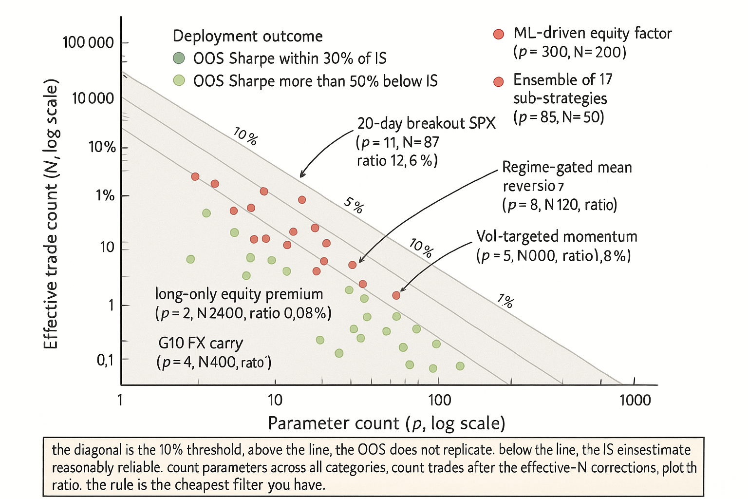
KEY POINTS

The 10% rule of degrees of freedom: the parameter count divided by the effective trade count should be at most 10%. A ratio of 1-3% is preferred. A ratio of 5-10% requires bias-corrected reporting alongside raw IS Sharpe. A ratio above 10% is in the "exploratory only" zone.
The structural justification: the standard error of an IS Sharpe estimate with N trades is approximately 1/sqrt(N), the bias from optimization across p parameters scales with sqrt(p), and the bias-to-noise ratio scales with sqrt(p N). The 10% threshold corresponds to a bias-to-noise ratio of approximately 1.
The parameter count p is the eight-category total from "Degrees of Freedom in Trading Systems": numeric grids, structural choices, filters and gating, sizing schemes, market and time-period selection, cost assumptions, data choices, abandoned-strategy selection.
The effective trade count N is the number of independent realizations of per-trade P&L, not the total observation count. Subtleties: hold-time overlap (effective N approximately observations divided by hold time), cross-sectional position dependence (effective N approximately rebalance count for long-short factor strategies), regime-conditional trades (effective N is the trade count within the gating regime).
When the ratio is too high, the typical fix is to reduce p, not to extend N. Reducing p is usually faster, cheaper, and more effective than extending N.
Three scenarios for ratio violations: small N strategies need extension or removal of parameters, large N strategies with high p need parameter pruning, very small N strategies are exploratory and should not be deployed at scale regardless of p.
The rule does not certify a strategy. A low ratio is necessary but not sufficient; a high ratio is a red flag but not an automatic rejection. The rule informs the deployment gating in combination with structural premise, regime coverage, and OOS validation.
Anti-pattern: counting only the visible numeric parameters. The full-category p is typically 5-10x the visible count.
Anti-pattern: counting position-observations as trades. Effective N corrects for hold-time overlap and cross-sectional dependence.
Anti-pattern: applying the rule as a binary filter rather than as a quantitative input. The right application: report ratio for every strategy, report bias-corrected Sharpe, gate deployment based on combined diagnostics.
Anti-pattern: ignoring the rule on "structural" strategies. The structural prior choices are still DoFs.
Anti-pattern: treating the rule as a substitute for OOS testing. The rule informs the IS-OOS gap expectation; the OOS check is the actual validation.
The current article gives the quantitative threshold for parameter-to-trade ratios. The next article in the publication ("Trade-Count Thresholds for Backtest Reliability") gives the absolute trade-count requirements that complement the relative ratio.