3. Robust Systems Lab May 28, 2026 10 min

3.16 Degrees of Freedom in Trading Systems

Eight DoF categories, with numeric parameters as one of them. A "simple" strategy often hides thousands or millions of configurations. Count them all, apply the bias correction.

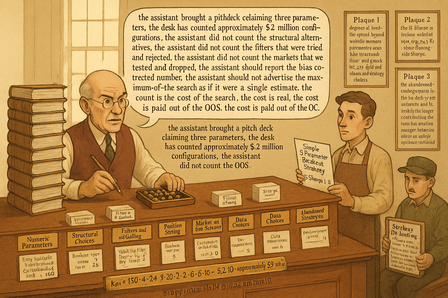
A retail trader presents a system at a conference. The pitch: "a simple breakout strategy on SPX futures. Buy when price closes above the 20-day high. Exit when price closes below the 10-day low. Position size based on 14-day ATR. The IS Sharpe is 1.8 over 2010-2020." The audience hears "simple" and counts what they consider the parameters: lookback for entry (20), lookback for exit (10), ATR period (14). Three parameters. Sounds reasonable. The system is purchased by a small fund and deployed in 2021. The OOS Sharpe through 2024 is approximately 0.2.

The post-mortem reveals the actual degrees of freedom. The breakout type was chosen (close-above-N-high vs intraday-above-N-high vs Donchian-channel vs ATR-buffered-breakout) - that is one binary or categorical choice across at least four candidates. The entry lookback (20) was selected from a small grid that the trader admits considering values of 10, 15, 20, 25, 30, and 40 - that is a 6-way choice. The exit lookback (10) was similarly chosen from {5, 7, 10, 14, 20} - a 5-way choice. The ATR period (14) is a 5-way choice from common values {7, 10, 14, 20, 28}. The position-sizing scheme was chosen (raw ATR vs ATR scaled by equity vs ATR scaled by 5-day average ATR) from at least three candidates. The market choice (SPX futures) was made from at least 5 liquid index futures (SPX, NDX, RTY, NIKKEI, EURO STOXX). The time period (2010-2020) was chosen rather than (2000-2010) or (1995-2010) or (2005-2015), each of which would have produced different IS Sharpes. The "no costs" framing was a methodological choice. The "no overnight gap risk" was unstated but implicit. The "no slippage above one tick" was an assumption.

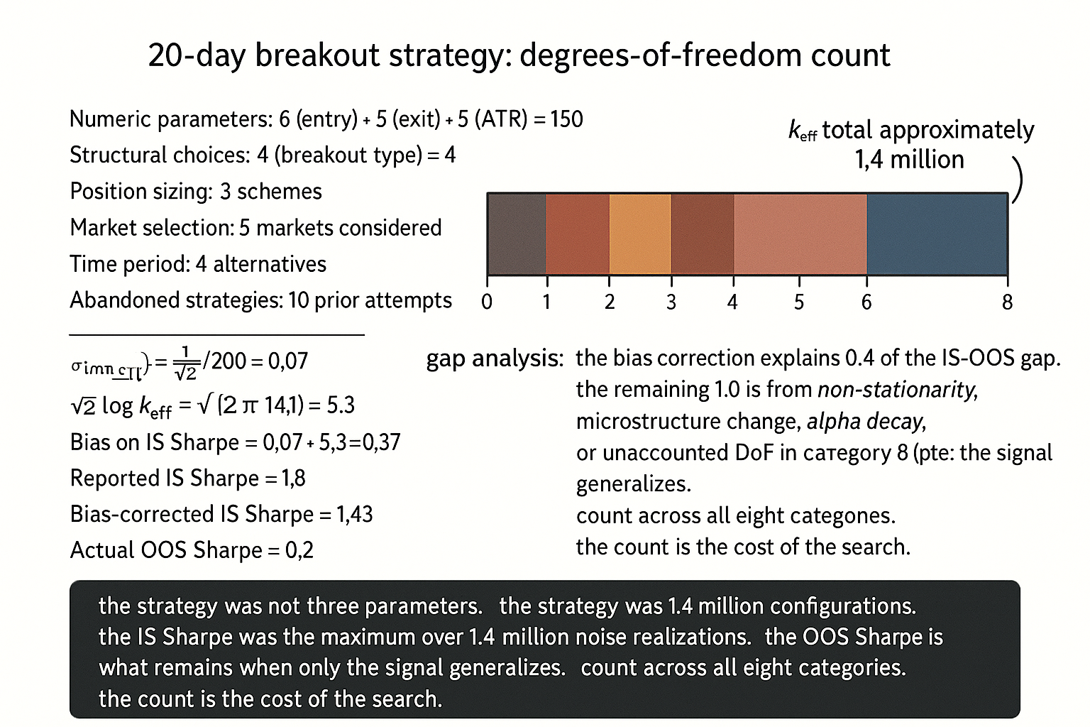
The actual degree-of-freedom count is approximately 4 (breakout type) x 6 (entry lookback) x 5 (exit lookback) x 5 (ATR period) x 3 (sizing scheme) x 5 (market choice) x 4 (time period) x 2 (cost assumption) = 144000 effective candidate configurations. The trader explored, consciously or unconsciously, a substantial fraction of this space and reported the maximum. The IS Sharpe of 1.8 was the maximum of approximately 144000 noise-plus-signal realizations; the OOS Sharpe of 0.2 is what remains when only the signal generalizes. The strategy was never "three parameters". It was thousands of effective parameters, dressed in a presentation that hid most of them. This article gives the framework for counting degrees of freedom without omission, so that the search-width bias from "The Difference Between Robustness and Optimization" can be made quantitative.

Counting degrees of freedom

Eight categories, often hidden.

Category 1: explicit numeric parameters. The lookback windows, thresholds, ATR multipliers, vol-target levels, stop-loss levels, take-profit levels. These are the visible degrees of freedom. The discrete grid the researcher considered (e.g., entry lookbacks from 10 to 40 in steps of 5) is the relevant search width, not the single value reported.

Category 2: structural choices. Indicator type (RSI vs MACD vs ROC vs custom), entry rule type (breakout vs mean reversion vs crossover vs filter), exit rule type (time stop vs price stop vs ATR stop vs signal reversal). Each structural choice is a categorical degree of freedom with cardinality equal to the number of candidates the researcher considered.

Category 3: filter and gating choices. "Only trade when 200-day MA is rising". "Only trade in volatility regime X". "Skip the first and last 30 minutes of the session". "Skip the day before and after FOMC". Each filter is a degree of freedom whose presence/absence and parameterization were chosen from candidates.

Category 4: position-sizing and risk-management choices. Fixed-size vs vol-targeted vs Kelly-fraction vs equity-curve-trailing. Each scheme has parameters (vol target, lookback, scaling factor). The choice of scheme and the values are degrees of freedom.

Category 5: asset universe and market selection. Which markets are included, which excluded, which time period is used as IS, which as OOS. Each inclusion/exclusion decision is a degree of freedom. The article "Why Works on All Markets Is Usually a Red Flag" framed the cross-market overfitting; the present article frames the same problem as a degrees-of-freedom count.

Category 6: cost and execution assumptions. Per-trade commission, slippage assumption (linear vs square-root vs ATR-scaled), bid-ask treatment (mid-price vs full spread vs realistic fills). The choice of assumption is a degree of freedom that often shifts the IS Sharpe by 20-50% in either direction.

Category 7: data choices. Bar interval (5-minute vs 15-minute vs hourly vs daily), data source (free vs licensed, vendor A vs vendor B), corporate-action handling (split-adjusted vs total-return vs dividend-reinvested), survivorship handling (current-constituents vs historical-constituents). Each is a degree of freedom.

Category 8: implicit constraints from researcher behavior. The strategy was not the first idea tried. Earlier ideas were abandoned and a new one tried. The researcher's selection across abandoned strategies is a degree of freedom that does not appear in the final report. This is the hardest category to count and is where most retail and small-shop research underestimates by an order of magnitude.

Counting effective degrees of freedom

The total effective DoF is approximately the product of the cardinalities across all eight categories (or the sum if you prefer log-space arithmetic). The relevant statistic is k_eff, the effective number of independent configurations the researcher could have reported.

$$ k_{\text{eff}} = \prod_{i=1}^{C} n_i, \qquad \text{Bias}_{\text{IS}} \approx \sigma_{\text{IS}} \cdot \sqrt{2 \log k_{\text{eff}}} $$

For the breakout-strategy example above: k_eff approximately 144000, sqrt(2 log 144000) approximately 4.9. The bias on the IS Sharpe estimate is approximately 4.9 standard errors. With N=200 trades, sigma_IS approximately 1/sqrt(200) approximately 0.07, the bias is approximately 0.34. The reported IS Sharpe of 1.8 implies a bias-corrected expected OOS Sharpe of approximately 1.5; the actual OOS of 0.2 suggests the bias correction is even larger because the configuration count was probably higher than 144000 once Category 8 (researcher selection across abandoned strategies) is included.

The full counting principle. List every choice that was made, including the choice "not to" do something (e.g., "we did not include FOMC-day filtering" is a choice that could have gone the other way). For each, count the number of alternatives the researcher considered. Multiply. The product is k_eff. The bias-corrected IS Sharpe is the reported IS Sharpe minus the search-width bias. Report both numbers, not the reported number alone.

The DoF count vs the headline number

Three structural reasons.

Reason 1: the IS Sharpe inflates with k_eff. The reported IS Sharpe is the maximum over k_eff noisy realizations of the true Sharpe. The expected gap between the reported maximum and the true Sharpe scales with sqrt(2 log k_eff). For k_eff = 100, the gap is approximately 3 standard errors. For k_eff = 10000, approximately 4 standard errors. For k_eff = 1000000, approximately 5 standard errors. The IS Sharpe is meaningless without k_eff in the denominator.

Reason 2: the OOS test loses statistical power as k_eff grows. The OOS test is meant to be an independent validation, but the test was implicitly part of the researcher's selection process if the researcher iterated until the OOS validated. The article "Why OOS Failure Is Often a Stationarity Failure" framed one cause of OOS failure; another cause is the OOS being implicitly part of the IS through the researcher's iteration process.

Reason 3: communication standards. A research team's discipline can be assessed by whether the team reports k_eff alongside the IS Sharpe. A team that reports "Sharpe 1.8 from 3 parameters" is either deceptive or has not counted across all categories. A team that reports "Sharpe 1.8 from approximately 10000 effective configurations, bias-corrected estimate 1.4" is forthright. The latter is rare; the former is common.

Practical counting protocol

Five steps to a defensible count.

Step 1: list every numeric parameter and the grid considered. Even values "tried briefly and rejected" count. If the researcher's brain tried entry lookbacks 5, 10, 15, 20, 25, 30, 40, 60 before settling on 20, the count for that parameter is 8, not 1.

Step 2: list every structural choice and the candidates. "We chose breakout over RSI; we considered Donchian vs ATR-buffered." Each enumerated alternative is a candidate.

Step 3: list every filter and gating choice (Category 3). Each filter applied or not applied, with its parameter grid.

Step 4: list every implicit choice from Categories 5-7 (markets, costs, data). Conservative count: assume at least 2-3 alternatives were considered for each implicit choice.

Step 5: estimate Category 8 (selection across abandoned strategies). If the researcher tried 10 different strategies before settling on the final one, the effective k is multiplied by 10 because the final strategy is the maximum over the 10 abandoned attempts as well as the within-strategy parameter search.

Multiply. Report k_eff. Apply the bias correction.

Anti-patterns

Five mistakes specific to DoF counting.

Anti-pattern 1: counting only the explicit numeric parameters. The breakout strategy has approximately 10000-100000 effective configurations once structural, filtering, sizing, market, and cost choices are included, far above the advertised "3 parameters".

Anti-pattern 2: ignoring the abandoned-strategy selection. The researcher tried 10 strategies and reports the best one. The implicit search width is multiplied by 10. The headline Sharpe of the best strategy is biased upward by the corresponding amount.

Anti-pattern 3: claiming "we did not optimize" when the parameters came from a structural prior. If the parameters are from the academic literature and not adjusted by the researcher, the within-strategy DoF is zero. But the strategy choice itself (which paper to follow, which parameters from which paper, which market to apply to) is still a DoF that needs to be counted.

Anti-pattern 4: treating k_eff and bias correction as theoretical concerns. The bias is real, predictable, and quantifiable. The bias-corrected IS Sharpe is the right number to use for OOS expectation. Skipping the bias correction is the same as skipping the OOS test.

Anti-pattern 5: reporting per-parameter sensitivity instead of total k_eff. Showing that "the strategy is robust to entry lookback in the range 15-25" is necessary but not sufficient. The total k_eff includes the choice of "entry-lookback as the parameter to vary" rather than other parameters. The robustness to one parameter does not imply robustness across all DoF.

Decision matrix

DoF category	Typical count per strategy	Reporting requirement
Numeric parameters	3-15 each, total 50-1000	Report grid considered, not single value
Structural choices	2-10 each, total 5-50	Enumerate candidates considered
Filters and gating	0-10 filters, each 2-5 candidates	List all filters, including absences
Sizing and risk-management	3-10 candidates total	Enumerate alternatives considered
Market and time-period selection	2-20 candidates	Justify selection and the alternatives considered
Cost and execution assumptions	2-5 candidates	Report sensitivity to cost assumption
Data choices	2-10 candidates	Report sensitivity to data source
Abandoned-strategy selection	1 to 50+	Report number of strategies tried before this one
Total k_eff	10000 to 10^9 typical	Report bias-corrected IS Sharpe alongside raw

The matrix is operational. The pattern: count across all categories, report k_eff, apply bias correction.

Visualizing degrees of freedom

KEY POINTS

Degrees of freedom in a trading system extend beyond the explicit numeric parameters. Eight categories: numeric parameters, structural choices, filters and gating, position sizing, market and time-period selection, cost and execution assumptions, data choices, abandoned-strategy selection.
The total effective DoF count k_eff is approximately the product of the cardinalities across all categories. A strategy advertised as "three parameters" typically has k_eff between 10000 and 10 million once all categories are counted in full.
The IS Sharpe is biased upward by approximately sigma_IS times sqrt(2 log k_eff). For k_eff = 1.4 million and sigma_IS = 0.07, the bias is approximately 0.37 Sharpe units. The bias-corrected IS Sharpe is the reported IS Sharpe minus this amount.
The bias-corrected IS Sharpe is the right number for OOS expectation. Skipping the bias correction is methodologically equivalent to skipping the OOS test. Reporting only the raw IS Sharpe is misleading.
A typical breakdown for a "simple" strategy: 50-1000 numeric configurations, 5-50 structural alternatives, 0-10 filters with their candidates, 3-10 sizing schemes, 2-20 market choices, 2-5 cost assumptions, 2-10 data choices, 1-50 abandoned prior strategies. Multiplied: 10000 to 10^9 effective configurations.
The hardest category to count is abandoned-strategy selection. The researcher tried 10 strategies before settling on the reported one. The reported strategy is the maximum over the 10 abandoned attempts as well as the within-strategy search; the implicit search width includes the 10x.
Anti-pattern: counting only the visible numeric parameters and reporting the strategy as "three parameters". The strategy is the visible parameters multiplied by the structural, filtering, sizing, market, cost, data, and abandoned-strategy choices.
Anti-pattern: ignoring the abandoned-strategy DoF. The researcher's brain searched across rejected strategies; the search width is multiplied accordingly.
Anti-pattern: claiming "we did not optimize" when the parameters came from a structural prior. The structural prior eliminates within-strategy DoF, but the choice of which structural prior to use is itself a DoF.
Anti-pattern: reporting per-parameter sensitivity as proof of low DoF. Robustness to one parameter is necessary but not sufficient; total k_eff includes the choice of which parameter to test.
The reporting standard: list every choice with the number of alternatives considered, multiply to get k_eff, apply the bias correction. Report both the raw IS Sharpe and the bias-corrected IS Sharpe. The latter is the OOS expectation.
The current article gives the counting framework. The next article in the publication ("Why More Parameters Make a Strategy Easier to Sell and Easier to Break") covers the marketing-vs-engineering trade-off that follows from the count.