3.23 CSCV: A Direct Probability of Backtest Overfit
PBO is the probability the IS-optimal parameter ranks below median OOS. CSCV enumerates all S-of-2S splits. Under 0.10 is robust; over 0.50 is pure overfit. Read the histogram, not the number.
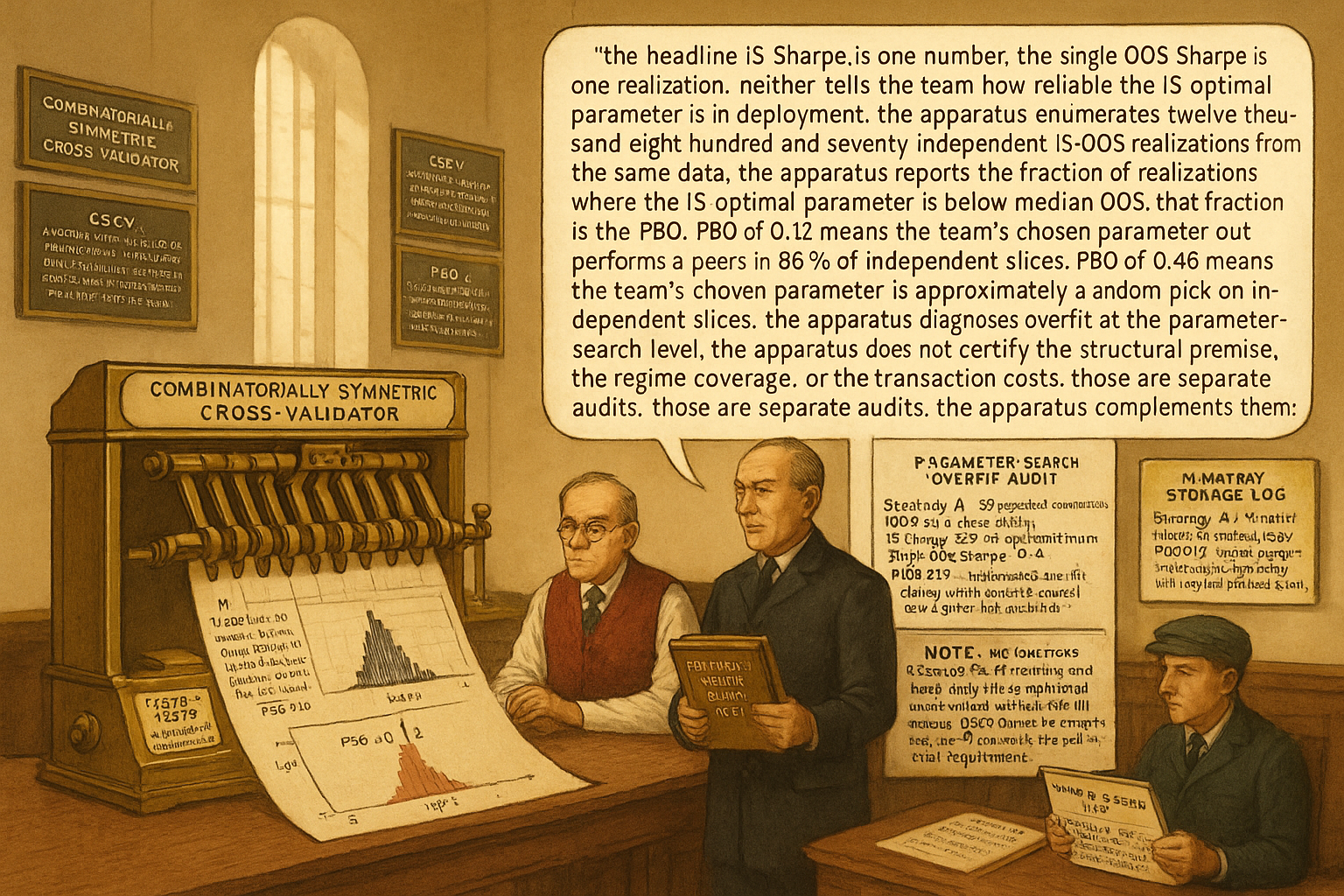
A research team optimizes a strategy across 50 candidate parameter sets, picks the IS-best, reports the IS Sharpe of 1.7, and runs an OOS hold-out that produces a Sharpe of 0.4. The team's question: was the OOS Sharpe of 0.4 a bad sample (the strategy is good but the OOS slice was unfortunate), or was the IS Sharpe of 1.7 the bad sample (the strategy is overfit and the OOS reveals the true capacity)? The standard methods covered earlier in this pillar give partial answers. The article "Degrees of Freedom in Trading Systems" gave the search-width bias formula. The article "Trade-Count Thresholds for Backtest Reliability" gave the standard error of the Sharpe estimate. Neither of them, by itself, tells the team how likely the strategy was to be overfit given the specific search the team performed.
The Probability of Backtest Overfitting (PBO), computed via Combinatorially Symmetric Cross-Validation (CSCV), gives a direct numerical answer. PBO is defined as the probability that the IS-optimal parameter set, evaluated on a different slice of data, performs below the median of all candidate parameter sets evaluated on that slice. A PBO of 0.5 means the IS-optimal parameter is no better than a random pick on out-of-sample data; a PBO of 0.05 means the IS-optimal parameter outperforms its peers on out-of-sample data. The number is computed mechanically from the strategy's per-period return series for each candidate parameter set, without requiring assumptions about the return distribution or the specific candidate-set geometry.
CSCV is a procedure that computes PBO from a matrix of per-period returns by parameter set. The procedure is mechanical, requires no calibration, and produces a single number that diagnoses the overfit risk specific to the search the team performed. This article gives the procedure step by step, the operational interpretation, and the legitimate uses and failure modes.
CSCV in one paragraph
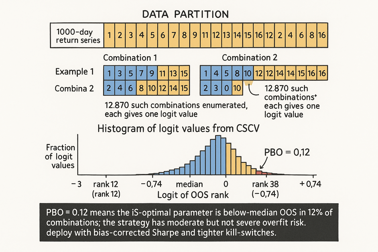
The data is a T-by-K matrix M, where T is the number of time periods and K is the number of parameter sets that were tried during the optimization. The matrix entry M[t, k] is the return of parameter set k in period t. CSCV splits the T time periods into 2S equal-size blocks (S blocks for IS, S blocks for OOS), with all S-of-2S combinations enumerated. For each combination, the IS-optimal parameter k is found by optimizing the Sharpe (or any other rank statistic) on the IS half. The OOS performance of k is then ranked among the OOS performances of all K parameter sets. The OOS rank is mapped to a "logit" via log(rank / (K + 1 - rank)). The full distribution of logit values across all combinations is the relative-overfit distribution. The PBO is the fraction of combinations where the IS-optimal parameter has below-median OOS rank, equivalent to the fraction of negative logit values.
The mechanical procedure removes the dependence on a single arbitrary IS-OOS split. The combinatorial enumeration produces many independent IS-OOS realizations from the same dataset, capturing the variability that the single-split design misses.
The procedure step by step
Six steps with concrete numbers from the example.
Step 1: build the M matrix. The strategy's K = 50 candidate parameter sets are run on the same T = 1000 daily-return periods. The M matrix has 50 columns and 1000 rows. Each cell M[t, k] is the daily return of parameter set k on day t.
Step 2: choose S. S is the number of blocks per half (so there are 2S blocks total). Common choices are S = 8 (16 blocks total, 12870 combinations of S-out-of-2S) or S = 6 (12 blocks total, 924 combinations). Larger S gives more combinations but smaller blocks; smaller S gives fewer combinations but larger blocks. S = 8 is the standard choice for daily data with several years of history.
Step 3: enumerate combinations. For 2S = 16 blocks, the number of S-out-of-2S combinations is C(16, 8) = 12870. Each combination J selects 8 blocks for IS and the remaining 8 for OOS.
Step 4: for each combination J, compute the IS-best parameter. Compute the Sharpe of each of the 50 parameter sets on the 8 IS blocks. Find k* = argmax_k Sharpe_IS(k).
Step 5: rank the OOS performance of k. Compute the Sharpe of each of the 50 parameter sets on the 8 OOS blocks. Rank them. Find the rank r of k among the 50 OOS Sharpes (r between 1 and 50).
Step 6: compute the logit. The OOS-rank logit is log(r / (51 - r)). A logit of 0 means k has median OOS rank (rank 25 or 26 of 50). A negative logit means k has below-median OOS rank (the IS-optimal parameter is worse than half of its peers OOS). A positive logit means above-median.
Repeat steps 4-6 for all 12870 combinations. The empirical distribution of logits across combinations is the CSCV result. The PBO is the fraction of combinations with logit < 0.
$$ \text{PBO} = \frac{1}{|\mathcal{J}|} \sum_{J \in \mathcal{J}} \mathbb{1}\left\{ \text{rank}_{\text{OOS}}^{(J)}(k^*_{\text{IS}}^{(J)}) < \tfrac{K + 1}{2} \right\} $$
The set J is the set of all S-of-2S combinations.
Reading the PBO number
Operational interpretation calibrated against published practice and observed deployment outcomes.
PBO < 0.10: the IS-optimal parameter robustly outperforms its peers on independent slices. The strategy is not overfit at the parameter-search level; the IS Sharpe is approximately the true Sharpe minus modest sampling noise. Deploy.
PBO 0.10-0.30: moderate overfit risk. The IS-optimal parameter is better than median on most slices but not all. The IS Sharpe is moderately inflated. Deploy with smaller capital, tighter kill-switches, and the bias-corrected Sharpe from "Degrees of Freedom in Trading Systems".
PBO 0.30-0.50: high overfit risk. The IS-optimal parameter is approximately equivalent to a random pick on independent slices. The IS Sharpe is mostly noise. Do not deploy without further reduction in parameter count or extension of the data.
PBO > 0.50: the IS-optimal parameter is below median on most slices. The IS Sharpe is purely from search-width inflation. The strategy has no detectable edge. Reject.
The thresholds are heuristic. The published research on CSCV calibrates against historical strategies with known OOS outcomes; the rough mapping above is consistent with the published guidance. Different strategy families may have different operational thresholds (high-Sharpe-true strategies have lower PBO at any given search width; low-Sharpe-true strategies have higher PBO).
CSCV vs a single OOS split
Three structural advantages.
Advantage 1: many IS-OOS realizations from the same data. The single-OOS-split design produces one realization of the OOS Sharpe. The CSCV design produces 12870 realizations (for S = 8). The variance across realizations reveals the strategy's true sensitivity to which slice is held out. A strategy with PBO 0.45 has high realization-to-realization variance: depending on which slice is held out, the IS-optimal parameter looks like the best or worst pick. A strategy with PBO 0.05 has low variance: the IS-optimal parameter is consistently good across slices.
Advantage 2: no arbitrary split choice. The single-OOS design depends on the choice of IS-OOS boundary (e.g., 70-30 vs 80-20 vs the 2018 break point). Different boundaries can produce different OOS results, and the team's incentive is to choose the boundary that produces the best result. CSCV averages over all combinations, removing the boundary-selection degree of freedom.
Advantage 3: measures overfit at the parameter-set level, beyond OOS performance on one slice. A single OOS split tells you the OOS Sharpe of one parameter set on one slice. CSCV tells you the relative rank of the IS-optimal parameter compared to its peers on independent slices. The relative-rank statistic is more robust to overall-strategy-quality variation across slices and isolates the overfit-specific risk.
Data requirements for CSCV
Three requirements. Failures of any one make CSCV results unreliable.
Requirement 1: per-parameter return time series for all K candidates. The CSCV procedure needs the full M matrix across all candidate parameter sets, beyond the IS-optimal parameter's track record alone. Many backtesting workflows save only the optimized result; CSCV requires re-running the strategy at all candidate parameter sets to populate M.
Requirement 2: enough data for meaningful blocks. With 2S = 16 blocks, T should be at least 16 times the autocorrelation horizon of the returns. For daily data with weekly autocorrelation, T should be at least 80 days; in practice, T should be at least 500 to make blocks of 30+ days.
Requirement 3: i.i.d.-like blocks. CSCV implicitly assumes the blocks are exchangeable. For strongly non-stationary data (the article "Slow Wandering: The Most Dangerous Type of Market Change" framed the problem), the blocks from different eras may have different mean and variance, and the rank-based statistics are still valid but the interpretation requires regime-aware reading. Combining CSCV with the regime stratification from "Regime Coverage: Why Your Backtest Needs Different Market States" gives a more robust diagnostic.
Cases where PBO disagrees with the OOS Sharpe
Three diagnostic patterns.
Pattern 1: IS Sharpe high, OOS Sharpe low, PBO low (< 0.15). The strategy is sound but the chosen OOS slice is unrepresentative (e.g., a single regime that the strategy struggles in). The article "Why OOS Failure Is Often a Stationarity Failure" framed the regime-mismatch diagnosis. The CSCV result is the more reliable estimate of the strategy's true performance because it averages across many slices.
Pattern 2: IS Sharpe high, OOS Sharpe high, PBO high (> 0.40). The OOS slice happens to favor the IS-optimal parameter, but most other slices would not. The strategy has substantial overfit risk despite the favorable OOS realization. Do not deploy at full capital.
Pattern 3: IS Sharpe high, OOS Sharpe low, PBO high (> 0.40). The strategy is overfit on both the headline numbers and the CSCV diagnostic. Reject.
The PBO acts as a tiebreaker between the IS and the OOS. A low PBO supports the IS estimate; a high PBO supports skepticism even when the OOS happens to look good.
Anti-patterns
Five mistakes specific to CSCV and PBO.
Anti-pattern 1: computing PBO on a single parameter set. PBO requires the full K-by-T matrix; computing it on K = 1 is meaningless. The strategy must have multiple candidate parameter sets that were considered during research; if only one was considered, the PBO concept does not apply (and the search-width bias from "Degrees of Freedom in Trading Systems" is the right diagnostic).
Anti-pattern 2: cherry-picking the parameter set after seeing PBO. A team computes PBO with K = 50 candidates, finds PBO = 0.42 (high), drops some candidates to lower the PBO, and re-reports. The cherry-picking is itself a form of overfitting and inflates the apparent significance. The K should be fixed before computing PBO.
Anti-pattern 3: applying CSCV to optimization metrics other than Sharpe without checking sensitivity. The PBO depends on the choice of optimization metric. CSCV with Sharpe and CSCV with profit factor on the same strategy can give different PBO values. Report PBO under multiple metrics if the choice is not fixed by the strategy's deployment objective.
Anti-pattern 4: treating PBO as a complete certification. PBO measures overfit at the parameter-search level. It does not measure structural-premise validity (the article "Why Benchmarks Matter in Rule Evaluation" framed this requirement), regime coverage (the article "Regime Coverage: Why Your Backtest Needs Different Market States"), or transaction-cost realism. A strategy with PBO < 0.10 that ignores costs or has no structural premise is still bad.
Anti-pattern 5: reporting only the PBO without the underlying logit distribution. The full distribution of logits across combinations is informative beyond the binary PBO. A distribution heavily concentrated near zero suggests the IS-optimal parameter is not strongly preferred. A distribution with a clear positive mode (positive logit) suggests genuine ranking benefit. Report the histogram alongside the PBO.
Decision matrix
| PBO | Interpretation | Action |
|---|---|---|
| < 0.05 | IS-optimal parameter strongly outperforms peers OOS | Deploy at full capital |
| 0.05-0.15 | IS-optimal parameter robustly preferred | Deploy with standard monitoring |
| 0.15-0.30 | Moderate overfit risk | Deploy with smaller capital, tighter kill-switches |
| 0.30-0.50 | High overfit risk, IS-optimal is approximately random OOS | Do not deploy without parameter-count reduction |
| 0.50+ | IS-optimal is worse than median OOS | Reject; pure search-width artifact |
| Disagreement: low PBO, low OOS Sharpe | Trust CSCV; OOS slice unrepresentative | Investigate slice, redeploy |
| Disagreement: high PBO, high OOS Sharpe | Trust CSCV; OOS slice happens to favor | Reduce capital, more validation |
The matrix maps PBO range to action. The pattern: PBO is the headline overfit diagnostic; combine with the IS-OOS comparison and the structural-premise check.
Visualizing CSCV
KEY POINTS
- The Probability of Backtest Overfitting (PBO) is the probability that the IS-optimal parameter set, evaluated on an independent slice, performs below the median of all candidate parameter sets on that slice. PBO of 0.5 means the IS-optimal parameter is no better than a random pick OOS; PBO of 0.05 means it outperforms peers OOS.
- Combinatorially Symmetric Cross-Validation (CSCV) computes PBO mechanically from a T-by-K matrix M of per-period returns by parameter set. The procedure splits T into 2S blocks, enumerates all S-of-2S combinations, finds the IS-best parameter on each combination, ranks its OOS performance, and computes the fraction of below-median ranks.
- The OOS-rank statistic is converted to a logit via log(r / (K+1-r)). The full distribution of logits across combinations is the CSCV result. PBO is the fraction of negative logits.
- Operational thresholds: PBO < 0.10 = strong, deploy. 0.10-0.30 = moderate risk, deploy with smaller capital and kill-switches. 0.30-0.50 = high risk, do not deploy without parameter-count reduction. > 0.50 = pure search-width artifact, reject.
- Three structural advantages over a single OOS split: many IS-OOS realizations (12870 for S=8), no arbitrary boundary choice, directly measures relative overfit rather than absolute OOS performance.
- Three data requirements: per-parameter return series for all K candidates, enough data for meaningful blocks (T at least 16 times the autocorrelation horizon, in practice 500+ for daily), exchangeable-ish blocks (regime stratification helps for strongly non-stationary data).
- Three diagnostic patterns when PBO disagrees with raw OOS: low PBO + low OOS = trust CSCV, OOS slice unrepresentative, redeploy; high PBO + high OOS = OOS slice happens to favor, reduce capital; high PBO + low OOS = overfit confirmed, reject.
- Anti-pattern: computing PBO on a single parameter set. CSCV requires the full K-by-T matrix.
- Anti-pattern: cherry-picking K after seeing PBO. K must be fixed before computing.
- Anti-pattern: applying CSCV to one optimization metric without checking sensitivity. Report PBO under multiple metrics if the choice is not fixed by deployment objective.
- Anti-pattern: treating PBO as complete certification. PBO measures overfit at the parameter-search level only. Combine with structural-premise check, regime coverage, transaction-cost realism.
- Anti-pattern: reporting PBO without the logit-distribution histogram. The shape of the distribution is informative beyond the binary PBO.
- The current article gives the most direct overfit diagnostic available. The next article in the publication ("Why Walk-Forward Testing Is Better Than One Big OOS Split") covers a different validation technique that simulates real-time deployment cadence and complements CSCV's combinatorial approach.
References
- Testing and Tuning Market Trading Systems - Timothy Masters (Amazon)
- Data Mining Algorithms in C++ - Timothy Masters (Amazon)
- Tactical Investment Algorithms
- 1 Introduction - arXiv
- Refining and Robust Backtesting of A Century of Profitable Industry
- A Comprehensive Review of Statistical Methods in Quantitative
- Systematic Trend-Following with Adaptive Portfolio Construction
- Machine Learning in Quantitative Finance: A Systematic Review of
- SHARP: A Self-Evolving Human-Auditable Rubric Policy for ... - arXiv
- Full article: Enhanced Portfolio Optimization - Taylor & Francis