A trading rule's performance number, on its own, is meaningless. A strategy that returned 15% per year is excellent if the market returned 0%, mediocre if the market returned 14%, and embarrassing if the market returned 25%. The number 15% in isolation carries no information about whether the rule did anything useful. Information appears only when the rule is compared to a benchmark.

The choice of benchmark is the choice of what claim the rule is allowed to make. A bad benchmark turns a worthless rule into a publishable result. A good benchmark exposes the parts of the return that came from the rule and separates them from the parts that came from anything else.

Most retail backtests pick the worst possible benchmark (zero) and call the result evidence of edge. The result is the same long-biased momentum-tilted strategies dressed up as discoveries, year after year.

Everyone is a genius in a bull market

The cleanest statement of the benchmark problem: any rule that is long-biased during a period when the market drifted up will produce positive returns regardless of whether the rule itself has any predictive content.

A simple thought experiment. Take a roulette wheel and use it to generate buy and sell signals on the SPX over the past 25 years. The roulette wheel produces buys 60% of the time and sells 40% of the time. The roulette wheel has no predictive power. It is a roulette wheel.

The SPX drifted up at roughly 0.04% per day over that period. The roulette wheel, by virtue of being long more often than short, captures part of that drift. Its expected return under no predictive power is:

(0.60 × 0.04%) − (0.40 × 0.04%) = 0.008% per day ≈ 2% per year

Two percent per year of pure free return for a system that is randomness. A backtest of this roulette-wheel strategy, reported against a zero benchmark, would show "the strategy generates 2% per year over a 25-year sample." That sentence is true. The implication that the strategy is doing something is false.

The fix is to compare the rule against a benchmark that captures the same structural exposure as the rule but without any predictive content. The remainder, if positive, is what the rule actually contributed.

The bias-matched random rule

The cleanest benchmark for testing predictive timing is a random rule with the same long/short bias as the actual rule.

The expected return of a random rule that is long with probability P_L and short with probability P_S = 1 − P_L, on a market with average return μ_market per period, is:

This is the return the rule would produce purely from its directional bias interacting with the market's drift. It contains zero predictive content. Anything the actual rule generates above this number is the rule's predictive contribution.

The adjusted return of the rule, the part attributable to actual predictive power, is:

Worked example. A rule on the SPX from 2000 to 2024 spends 90% of the time long and 10% of the time short. The observed average daily return is 0.10%. The SPX drifted up at 0.05% per day over the same window.

Random rule expected return = (0.90 − 0.10) × 0.05% = 0.04% per day

Annualized random contribution = 0.04% × 252 ≈ 10%

Annualized observed return = 0.10% × 252 ≈ 25%

Adjusted return = 25% − 10% = 15%

The rule actually contributed 15 percentage points per year. The other 10 percentage points came from being long-biased in a market that went up. A backtest reported against a zero benchmark would claim 25%. A backtest reported against the bias-matched benchmark claims 15%. The two numbers describe different things, and the second one is the one that captures the rule's actual skill.

The hierarchy of benchmarks

Different benchmarks answer different questions. A complete evaluation uses several. From least to most informative:

Zero return. The naive benchmark. Useful only for market-neutral strategies that have no directional exposure. For any long-biased or short-biased rule, the zero benchmark is wrong because it credits the rule with returns that came from drift.

Risk-free rate. The floor any risky capital allocation must clear. A strategy that returns less than cash is a strategy that destroyed value. Useful as a hard minimum but rarely informative beyond that.

Buy-and-hold of the underlying. The relevant benchmark for any long-only strategy on a single asset. If a fund is long-only on the SPX and underperforms buy-and-hold SPX, the fund is destroying value relative to a no-effort alternative. Many published equity strategies fail this benchmark.

Bias-matched random rule. The benchmark for testing pure predictive timing. Strips out the contribution of directional bias × market drift. The cleanest test of whether the rule's signals carry information about future returns.

Peer strategies in the same class. The benchmark for competitive ranking. A trend-following strategy should be compared to other trend-following strategies (or to indices that track the trend-following industry). Outperforming the peer benchmark is the claim that the strategy is differentiated, not just that it works.

Factor model. The benchmark for risk-adjusted return. A regression of the strategy's returns on a set of factors (market, size, value, momentum, quality) decomposes the return into the part explained by known factors and the part that is unexplained. The unexplained part is the alpha. Any strategy whose returns can be fully explained by known factors is not adding value; it is delivering factor exposure that could be obtained more cheaply.

A rigorous evaluation reports the rule's performance against several of these benchmarks. The pattern of results tells the trader what the rule is actually doing.

Why the benchmark choice changes the conclusion

The same backtest can look excellent against one benchmark and worthless against another. This is not a flaw in the test. It is the point of the test.

Consider a long-biased trend-following rule on SPX over the past 15 years.

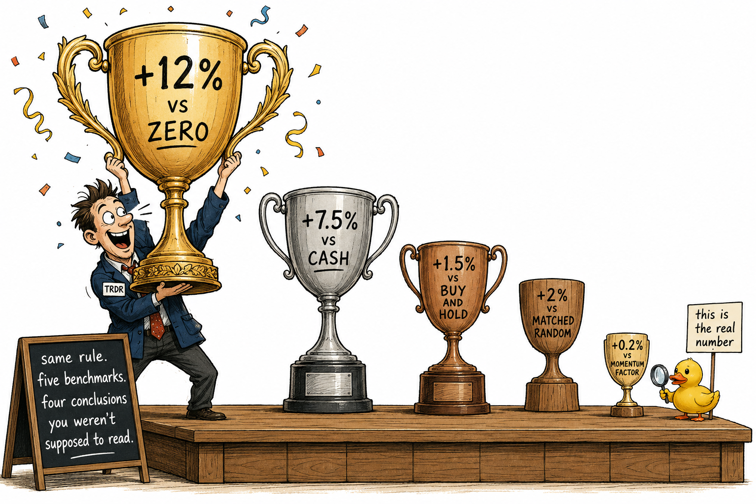
Against zero: 12% per year. Looks great.

Against buy-and-hold SPX: roughly flat. The rule captured the same drift the market captured.

Against a bias-matched random rule: marginal positive. The rule's specific timing added maybe 1% per year.

Against a momentum factor: roughly zero alpha. The rule's returns are mostly explained by exposure to the momentum factor, which is freely available through ETFs at low cost.

Same rule. Four benchmarks. Four conclusions. The honest report is all four numbers, not the one that flatters the rule. The dishonest report is the 12% against zero.

Visualizing the benchmark hierarchy

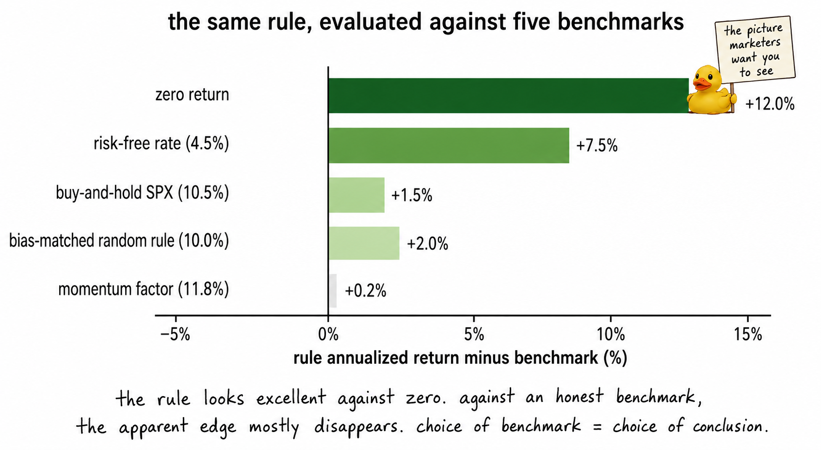
The visual is the essence of the benchmark problem. The same rule shrinks dramatically as the benchmark gets more honest. The marketer picks the leftmost bar. The honest evaluator reports all five.

The information ratio: a unified comparison

The information ratio extends the Sharpe ratio idea to performance relative to any benchmark. It is the Sharpe ratio computed on the difference between the rule's returns and the benchmark's returns.

The numerator is the mean excess return over the benchmark. The denominator is the standard deviation of that excess return. The IR is high when the rule consistently beats the benchmark by a stable margin. The IR is low when the rule occasionally beats the benchmark by a lot but is unreliable, or when the rule's average outperformance is small.

A strategy with a Sharpe ratio of 1.2 against zero and an information ratio of 0.1 against buy-and-hold is a strategy that captures drift, not edge. A strategy with a Sharpe ratio of 1.2 against zero and an information ratio of 1.0 against buy-and-hold is a strategy that genuinely beats the alternative on a risk-adjusted basis.

The IR against the right benchmark is the single number that summarizes whether a rule adds value. The Sharpe ratio against zero, in isolation, does not.

The retail mistake

Almost every retail backtest reports a single annualized return and a single Sharpe ratio, both computed against zero. This is the worst possible evaluation.

A few patterns recur in retail backtest claims:

A long-only SPX trend-following rule that beats zero by 12% but matches buy-and-hold gets sold as a 12% strategy. It is a 0% strategy.

A short-vol rule that pays steady 8% returns most of the time and blows up every few years gets sold as a high-Sharpe strategy against zero. Against a properly bias-matched benchmark that captures the same volatility-selling exposure, the alpha is negative.

A momentum strategy that returns 18% per year gets sold as a quant edge. Against the momentum factor, the alpha is zero. The strategy is delivering known factor exposure at a markup.

The benchmark fix in each case is simple and the conclusion changes completely. The strategy seller does not want the conclusion to change. The honest researcher does.

What this changes operationally

Three changes to standard practice.

Always report multiple benchmarks. At minimum: zero, the relevant buy-and-hold, and a bias-matched random rule. For institutional reporting, add a factor model. The pattern across benchmarks tells the reader what the rule is.

Pre-commit to which benchmark is the primary one. The primary benchmark is the one that matches the claim the rule is making. A market-timing rule's primary benchmark is the bias-matched random rule. A long-only equity rule's primary benchmark is buy-and-hold. A market-neutral rule's primary benchmark is the risk-free rate. Committing in advance prevents post-hoc benchmark shopping.

Report the information ratio against the primary benchmark, not just the Sharpe ratio against zero. The IR is the single number that compresses the evaluation into one digit. The Sharpe against zero is the number that flatters the rule.

KEY POINTS

• A trading rule's return in isolation is meaningless. Information appears only when the return is compared to a benchmark.
• Any long-biased rule in an upward-drifting market produces positive returns even with zero predictive content. The zero benchmark credits the rule for returns it did not generate.
• The bias-matched random rule benchmark strips out the directional-bias × market-drift contribution: E[R_random] = (P_L − P_S) × μ_market. Anything the actual rule generates above this is the predictive contribution.
• A worked SPX example with 90% long bias on a 0.05% drift yields 10% per year of free return from bias alone. A rule reporting 25% annualized has actually contributed 15%, not 25%.
• The hierarchy of benchmarks, from least to most informative: zero, risk-free rate, buy-and-hold of the underlying, bias-matched random rule, peer strategies in the same class, factor model.
• Different benchmarks answer different questions. A rigorous evaluation reports the rule's performance against several of them. The pattern across benchmarks shows what the rule is actually doing.
• The information ratio (Sharpe ratio of excess return over the benchmark) is the unified comparison metric. IR against the right benchmark is the single most informative number for the rule.
• The retail mistake is reporting one number against zero. Long-only trend strategies sold as 12% strategies are often 0% strategies against buy-and-hold. Momentum strategies sold as quant edge are often zero-alpha factor exposure.
• Operational fix: report multiple benchmarks, pre-commit to the primary benchmark before testing, report the IR against the primary benchmark alongside the Sharpe against zero.