3. Robust Systems Lab May 28, 2026 10 min

3.28 MAE/MFE Analysis: Seeing What Net Profit Hides

MAE is the largest unrealized loss; MFE the largest unrealized gain. Plots reveal what aggregates hide: bounceback rates, profit capture, exit timing. Compute before adding stops or profit targets.

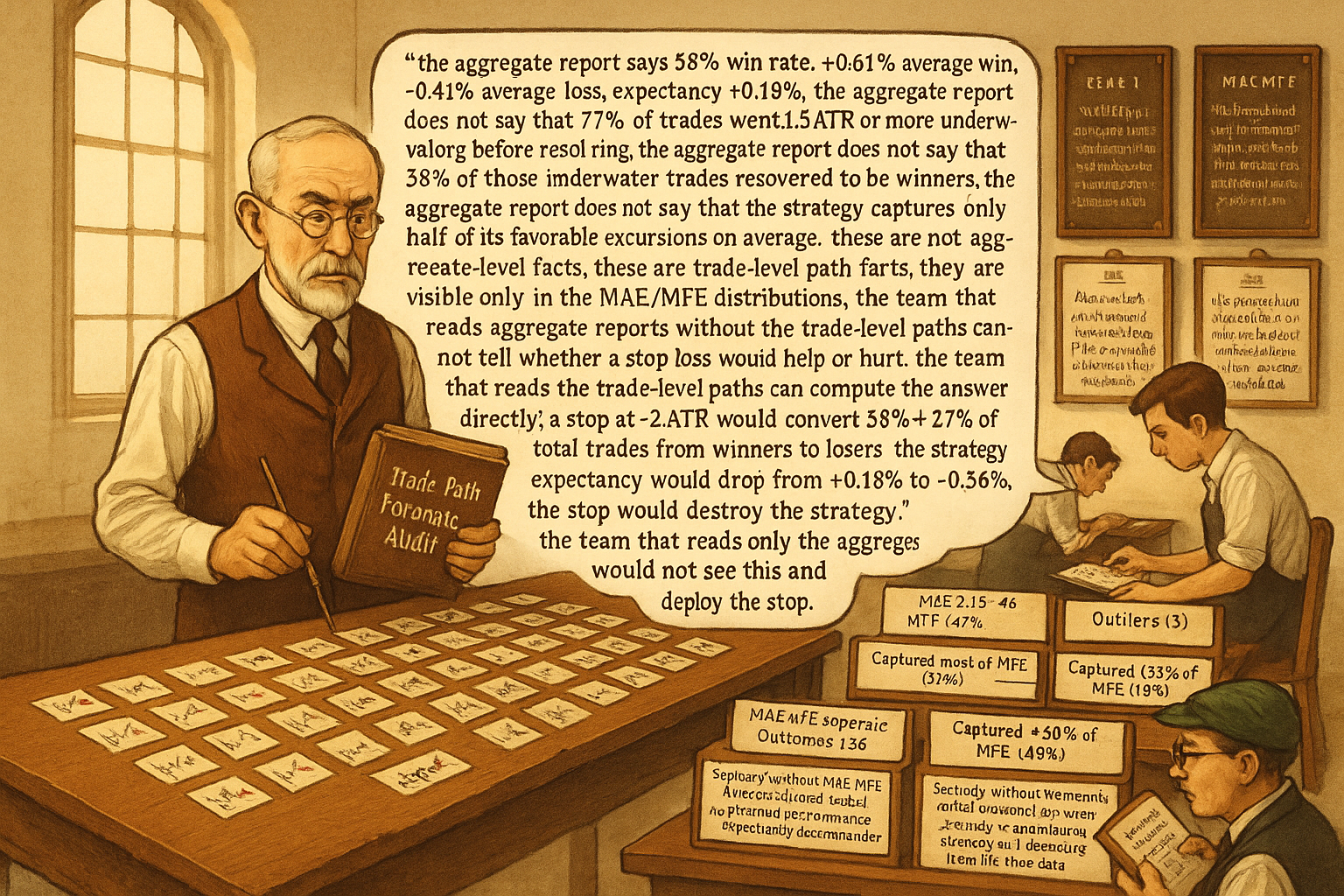
A breakout strategy on E-mini SPX has 320 trades over five years. The aggregate statistics: 58% win rate, average win +0.62%, average loss -0.41%, expectancy per trade +0.19%, annualized Sharpe 1.15, maximum drawdown 9.4%. The team is preparing to deploy. A junior researcher is asked to plot the Maximum Adverse Excursion (MAE) and Maximum Favorable Excursion (MFE) for each trade and look at the resulting scatter. The plots reveal patterns the aggregate statistics did not show.

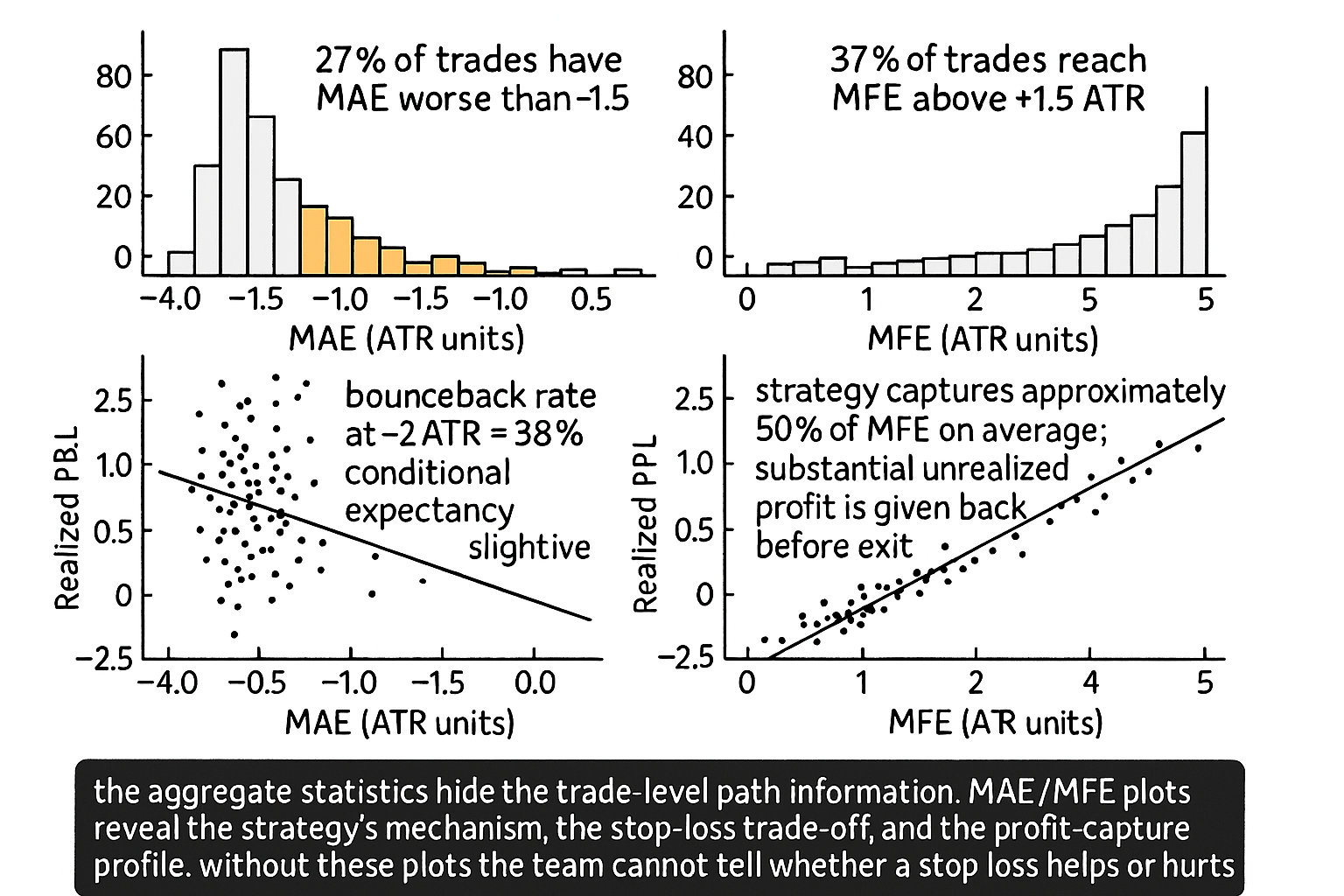
The MAE distribution: 31% of trades had an MAE between 0.0% and 0.5% (small adverse excursions, mostly winners). 42% had MAE between 0.5% and 1.5% (typical adverse range, mixed). 27% had MAE between 1.5% and 4.0% (large adverse excursions). Among the trades with MAE above 2%, 38% of them ended as winners (the position recovered) and 62% as losers (the position did not). The strategy regularly tolerates substantial adverse moves before recovering or being closed.

The MFE distribution: 14% of trades had MFE between 0.0% and 0.3% (no meaningful favorable move; mostly losers or quickly-stopped winners). 49% had MFE between 0.3% and 1.5% (modest favorable move that the strategy mostly captured). 37% had MFE between 1.5% and 5.0% (large favorable moves). Among the 37% with MFE above 1.5%, only 31% closed at their MFE level; the others closed at less than half of their peak favorable move. The strategy leaves substantial money on the table on its largest winners.

The aggregate statistics did not reveal either pattern. The 58% win rate told the team about the binary outcome but not about the path. The +0.62% average winner told the team about the realized profit but not about the unrealized profit that was given back. The -0.41% average loser told the team about the realized loss but not about the worst point during the trade. MAE/MFE analysis fills these gaps. The article "When a Stop Loss Improves Risk but Destroys Edge" framed the stop-loss trade-off; MAE/MFE is the diagnostic technique that quantifies which trades a stop-loss change would help or hurt before applying it. This article gives the framework, the standard plots, and the operational uses.

MAE and MFE, defined

Two trade-level statistics computed from the trade's price path.

MAE (Maximum Adverse Excursion). The largest unrealized loss the trade reached at any point during its life, measured in price units, percentage units, or ATR units. MAE is always non-positive (or zero, if the trade never went underwater). For a trade that opens long at 100, drops to 96, recovers to 102, and closes at 102, the MAE is -4 (or -4% if expressed as a percentage of entry).

MFE (Maximum Favorable Excursion). The largest unrealized gain the trade reached at any point during its life, measured in the same units as MAE. MFE is always non-negative. For the same example trade above, the MFE is +2 (or +2%).

Both statistics depend on the bar interval. For daily-bar backtests, MAE/MFE are computed from daily highs and lows. For minute-bar backtests, the resolution is finer and the MAE/MFE values are typically larger in magnitude (the intra-bar excursions are visible). The choice of bar interval is a degree of freedom that should be specified explicitly.

The standard MAE/MFE plots

Four plots, each diagnostic.

Plot 1: MAE histogram. Distribution of MAE values across all trades. The shape reveals how often the strategy goes underwater and by how much. A right-leaning distribution (most trades close to 0 MAE) suggests the strategy enters at favorable points; a left-leaning distribution (long tail of large negative MAE) suggests entries are often early and the strategy waits through adverse moves.

Plot 2: MFE histogram. Distribution of MFE values. A right-leaning distribution means most trades reach modest favorable levels; a heavy right tail means some trades reach large favorable levels. The shape reveals the strategy's profit-potential profile.

Plot 3: realized P&L vs MAE scatter. Each trade is a point with horizontal coordinate = MAE and vertical coordinate = realized P&L. The scatter shape reveals two things: (a) for trades with large MAE, what fraction recover to be winners (the "bounceback rate"), and (b) the typical P&L conditional on a given MAE level. For mean-reversion strategies, the scatter typically shows that trades with MAE in the -1 to -2 ATR range have higher win rates than trades with smaller MAE (counterintuitively, the trades that go underwater the most are the ones that recover). For trend-following strategies, the scatter typically shows the opposite: trades with large MAE are the ones that fail.

Plot 4: realized P&L vs MFE scatter. Each trade is a point with horizontal coordinate = MFE and vertical coordinate = realized P&L. The scatter reveals how much profit the strategy captures from its favorable excursions. A diagonal scatter (P&L approximately equal to MFE) means the strategy exits near its peak. A scatter where realized P&L is consistently below MFE (e.g., realized P&L is approximately 50% of MFE) means the strategy gives back substantial unrealized profit before closing.

Operational uses

Five direct applications.

Use 1: stop-loss design. The MAE distribution reveals where a stop loss would intervene. A stop at -2 ATR would close the 27% of trades with MAE > 2 ATR; if 38% of those would have recovered to winners (the bounceback rate from the MAE-vs-P&L scatter), the stop loss converts 38% * 27% = 10% of total trades from winners to losers. The expected change in expectancy from the stop loss is computable directly from the MAE distribution and the bounceback rate.

Use 2: profit-target design. The MFE distribution reveals where a profit target would intervene. A target at +1.5 ATR would close trades that reach +1.5 ATR before they continue to higher MFE. The realized-P&L-vs-MFE scatter shows what fraction of trades that reach +1.5 ATR continue to higher MFE versus reverse to lower realized P&L. For most trend-following strategies, the answer is "most continue", and the profit target costs more than it saves. For most mean-reversion strategies, the answer is "few continue", and the profit target captures profits that would otherwise be given back.

Use 3: entry-timing diagnosis. The MAE distribution at trade entry can be cross-tabulated with the entry signal's strength. If the strongest entry signals correspond to the smallest MAE (the strongest signals enter at the most favorable moments), the entry timing is well-calibrated. If the relationship is inverted (strong signals enter at the worst moments and tolerate large MAE), the entry timing has a problem.

Use 4: exit-timing diagnosis. The realized P&L vs MFE scatter quantifies the strategy's exit timing. A scatter where realized P&L is consistently below MFE by more than 50% indicates the strategy is exiting too late (giving back profits) or has stop losses that close trades on retracement before continuation. The article "When a Stop Loss Improves Risk but Destroys Edge" framed the stop-loss-related version of this; the MFE-based version applies more broadly.

Use 5: outlier identification. Specific trades with very large MAE or MFE that fall outside the typical distribution are outliers. They may correspond to specific market events (news shocks, gaps, microstructure events) that the strategy was not designed to handle. Investigating these outliers often reveals strategy specification gaps.

Limits of MAE/MFE

Three honest limits.

Limit 1: bar resolution. MAE/MFE on daily bars misses intraday excursions. A trade that opens long at 100, drops to 92 intraday, recovers to 99 by close, and closes at 99 next day shows MAE of -1 (close-to-close) on daily bars but MAE of -8 on intraday bars. The choice of bar resolution materially affects the MAE/MFE statistics.

Limit 2: causal vs anti-causal use. MAE/MFE are anti-causal statistics (computed from the full trade path including future bars). Using them for entry filtering would be look-ahead bias. They are appropriate for design analysis (where the trade path is known after the fact) but not for real-time entry signals.

Limit 3: small-sample noise. MAE/MFE distributions from a small number of trades (the article "Trade-Count Thresholds for Backtest Reliability" framed this) are noisy. The 27% / 38% bounceback rate in the opening example assumes 320 trades is enough; for 50 trades, the same statistics would have wide confidence intervals.

Anti-patterns

Five mistakes specific to MAE/MFE.

Anti-pattern 1: reporting only the aggregate statistics without the MAE/MFE plots. The aggregate statistics hide the trade-level path information. The MAE/MFE plots reveal patterns that determine whether stop losses, profit targets, or trailing stops would improve or destroy the strategy.

Anti-pattern 2: using MAE for real-time entry filtering. MAE is anti-causal; using it as if it were known at entry time is look-ahead bias.

Anti-pattern 3: setting stops at the IS-data MAE distribution boundary. The 95th percentile of the IS MAE distribution is one realization; the actual 95th percentile (across the larger population the IS sample is drawn from) is wider. Use bootstrap or synthetic-path Monte Carlo (covered in "Monte Carlo for Trading Systems") to estimate the operational MAE distribution.

Anti-pattern 4: ignoring bar resolution. Daily-bar MAE/MFE understate the actual intra-trade excursions for any strategy with hold time longer than one bar. Decide the bar resolution based on the strategy's monitoring cadence, not on the data convenience.

Anti-pattern 5: treating MAE/MFE as a strategy-improvement tool independent of structure. The patterns in the MAE/MFE plots reflect the strategy's mechanism. A stop loss that "fixes" the MAE distribution may break the underlying mechanism. Combine MAE/MFE diagnosis with structural understanding (covered in "Market Personality: Why Gold, FX, Crypto, and Equities Need Different Systems" and "When a Stop Loss Improves Risk but Destroys Edge").

Decision matrix

MAE/MFE pattern	Interpretation	Action
MAE distribution heavy in -1 to -2 ATR with high bounceback	Mean-reversion mechanism	No stop loss or wide stop
MAE distribution heavy in -2+ ATR with low bounceback	Trend-following mechanism	Stop at 2-3 ATR
MFE distribution diagonal scatter (realized P&L ~ MFE)	Exits near peaks	No profit target needed
MFE distribution with realized P&L << MFE	Strategy gives back profits	Trailing stop or earlier profit target
Strongest signals correlate with smallest MAE	Good entry timing	Continue
Strongest signals correlate with largest MAE	Entry timing problem	Investigate signal definition
Outlier trades with extreme MAE / MFE	Specification gap	Investigate per-event
Small sample (less than 100 trades)	High statistical noise	Add more data before drawing conclusions

The matrix maps MAE/MFE pattern to action. The pattern: the trade-level distribution is the diagnostic tool that aggregate statistics cannot replace.

The math of MAE-conditional expectancy

A useful calculation. The bounceback rate at a given MAE threshold M is the fraction of trades with MAE < -M that end as winners. The conditional expectancy at MAE threshold M is the average realized P&L of trades with MAE < -M.

$$ \text{Bounceback}(M) = \Pr(\text{P\&L} > 0 \mid \text{MAE} < -M), \qquad \text{Expectancy}(M) = \mathbb{E}[\text{P\&L} \mid \text{MAE} < -M] $$

For the opening example, Bounceback(2 ATR) approximately 0.38 and Expectancy(2 ATR) approximately +0.05% (the trades that go beyond 2 ATR adverse on average still end up positive by a thin margin). Adding a stop at -2 ATR would convert all of these trades from their actual outcome to a -2 ATR loss; the change in expectancy would be approximately Expectancy(2 ATR) - (-2 ATR) = +0.05% - (-2%) = -2.05% per affected trade, multiplied by the 27% of trades affected = -0.55% per total trade in expectancy. The strategy expectancy would drop from +0.19% to approximately -0.36%; the strategy would become unprofitable.

Visualizing MAE/MFE

KEY POINTS

Maximum Adverse Excursion (MAE) is the largest unrealized loss a trade reached during its life. Maximum Favorable Excursion (MFE) is the largest unrealized gain. Both are computed from the trade's price path; both depend on the bar resolution.
Four standard plots: MAE histogram, MFE histogram, realized P&L vs MAE scatter, realized P&L vs MFE scatter. Each reveals patterns that aggregate statistics cannot.
MAE distribution shape: right-leaning means trades enter at favorable points; left-leaning with long tail means entries are often early and the strategy waits through adverse moves. MFE distribution similarly diagnoses profit-potential profile.
P&L vs MAE scatter shows the bounceback rate (fraction of trades with large MAE that recover to be winners). For mean reversion, bounceback at -1 to -2 ATR is often higher than for smaller MAE. For trend following, the relationship inverts.
P&L vs MFE scatter shows profit capture. Diagonal scatter = strategy exits near peaks. Below-diagonal scatter = strategy gives back profits.
Five operational uses: stop-loss design (where the stop would intervene and what fraction of affected trades would have recovered), profit-target design (where the target would close and what fraction would continue), entry-timing diagnosis (cross-tabulate signal strength with MAE), exit-timing diagnosis (realized P&L vs MFE), outlier identification (specific trades with extreme excursions reveal specification gaps).
The MAE-conditional expectancy quantifies the impact of adding a stop loss at a given level. For the opening example, a -2 ATR stop reduces strategy expectancy by approximately 0.55% per total trade, converting a +0.19% strategy into a -0.36% strategy.
Three honest limits of MAE/MFE: bar resolution materially affects the values, the statistics are anti-causal so they cannot be used for real-time entry filtering, small samples (less than 100 trades) produce noisy distributions.
Anti-pattern: reporting only aggregate statistics without MAE/MFE plots. The plots are the diagnostic tool for path-dependent decisions.
Anti-pattern: using MAE for real-time entry filtering. MAE is anti-causal; using it for entry signals is look-ahead bias.
Anti-pattern: setting stops at IS-data MAE boundary without acknowledging it is one realization. Use bootstrap or synthetic paths for the operational distribution.
Anti-pattern: ignoring bar resolution. Daily MAE understates the actual intra-trade excursions for hold times longer than one bar.
Anti-pattern: treating MAE/MFE as a strategy-improvement tool independent of structure. The patterns reflect the mechanism; "fixing" the MAE distribution can break the underlying signal.
The current article gives the trade-level path diagnostic. The next article in the publication ("Why Profit Factor Can Lie") covers a different aggregate statistic that, like the headline net profit, hides important distributional information.